Generate a PCA plot.
Usage
get_pca_plot(
  x,
  samples = NULL,
  genes = NULL,
  circle_size = 10,
  label_replicates = FALSE,
  sample_colors = FALSE,
  sample.seed = 123
)
Arguments
- x
an abject of class "parcutils". This is an output of the function
run_deseq_analysis().- samples
a character vector denoting samples to plot in PCA plot, default
NULL. If set to NULL all samples are accounted.- genes
a character vector denoting genes to consider for PCA plot, default
NULL. If set to NULL all genes are accounted.- circle_size
a numeric value, default 10, denoting size of the circles in PCA plot.
- label_replicates
logical, default FALSE, denoting whether to label each replicate in the plot.
- sample_colors
a logical, default FALSE, denoting whether to shuffle colors of dots in PCA plot.
- sample.seed
an integer, default 123, denoting a value for
set.seed().
Examples
count_file <- system.file("extdata","toy_counts.txt" , package = "parcutils")
count_data <- readr::read_delim(count_file, delim = "\t")
#> Rows: 5000 Columns: 10
#> ── Column specification ────────────────────────────────────────────────────────
#> Delimiter: "\t"
#> chr (1): gene_id
#> dbl (9): control_rep1, control_rep2, control_rep3, treat1_rep1, treat1_rep2,...
#>
#> ℹ Use `spec()` to retrieve the full column specification for this data.
#> ℹ Specify the column types or set `show_col_types = FALSE` to quiet this message.
sample_info <- count_data %>% colnames() %>% .[-1] %>%
tibble::tibble(samples = . , groups = rep(c("control" ,"treatment1" , "treatment2"), each = 3) )
res <- run_deseq_analysis(counts = count_data ,
sample_info = sample_info,
column_geneid = "gene_id" ,
group_numerator = c("treatment1", "treatment2") ,
group_denominator = c("control"))
#> ℹ Running DESeq2 ...
#> converting counts to integer mode
#> Warning: some variables in design formula are characters, converting to factors
#> estimating size factors
#> estimating dispersions
#> gene-wise dispersion estimates
#> mean-dispersion relationship
#> final dispersion estimates
#> fitting model and testing
#> ✔ Done.
#> ℹ Summarizing DEG ...
#> ✔ Done.
get_pca_plot(x = res,sample_colors = TRUE) %>% print()
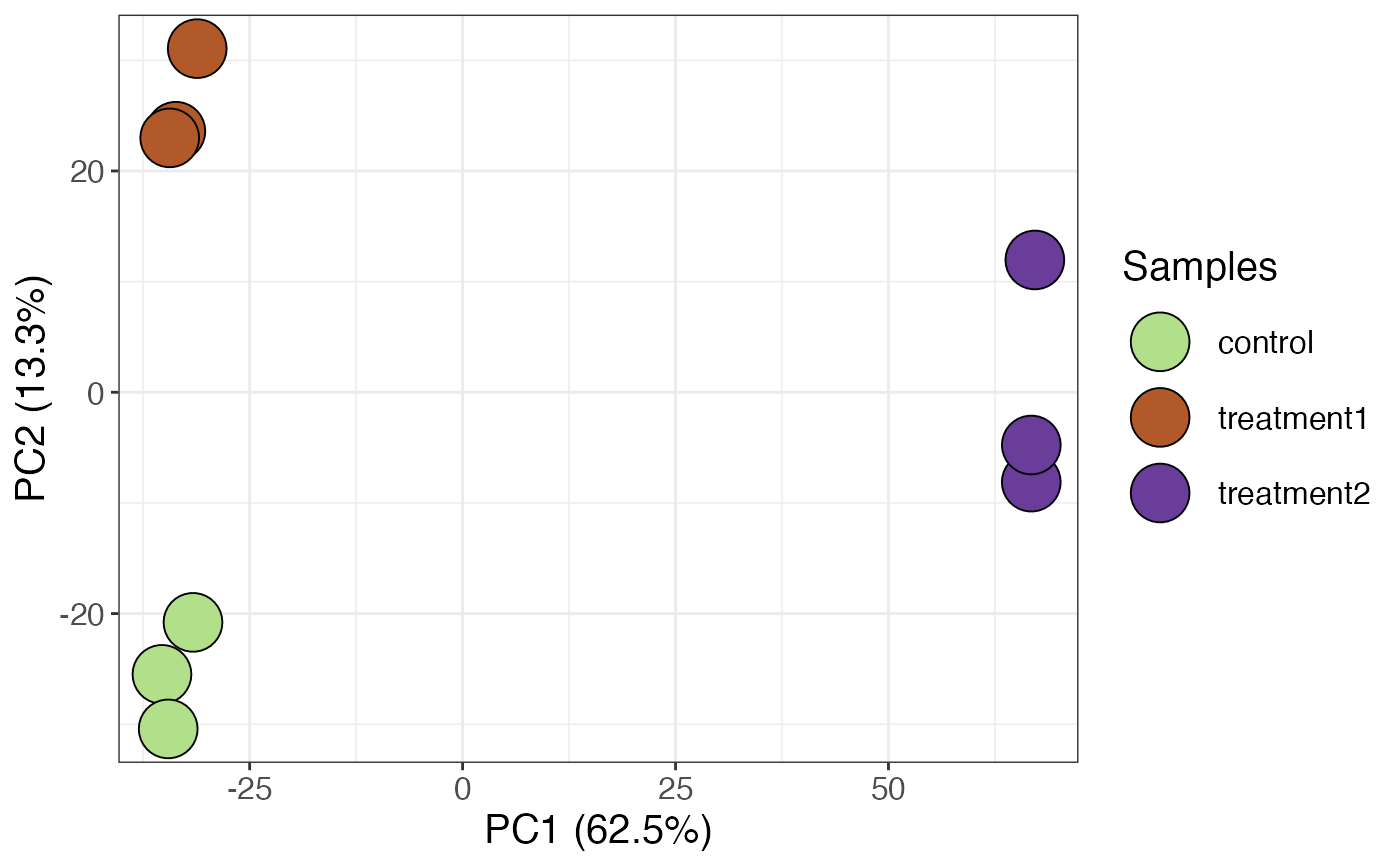 # reproduce sampled colors with argument `sample.seed`
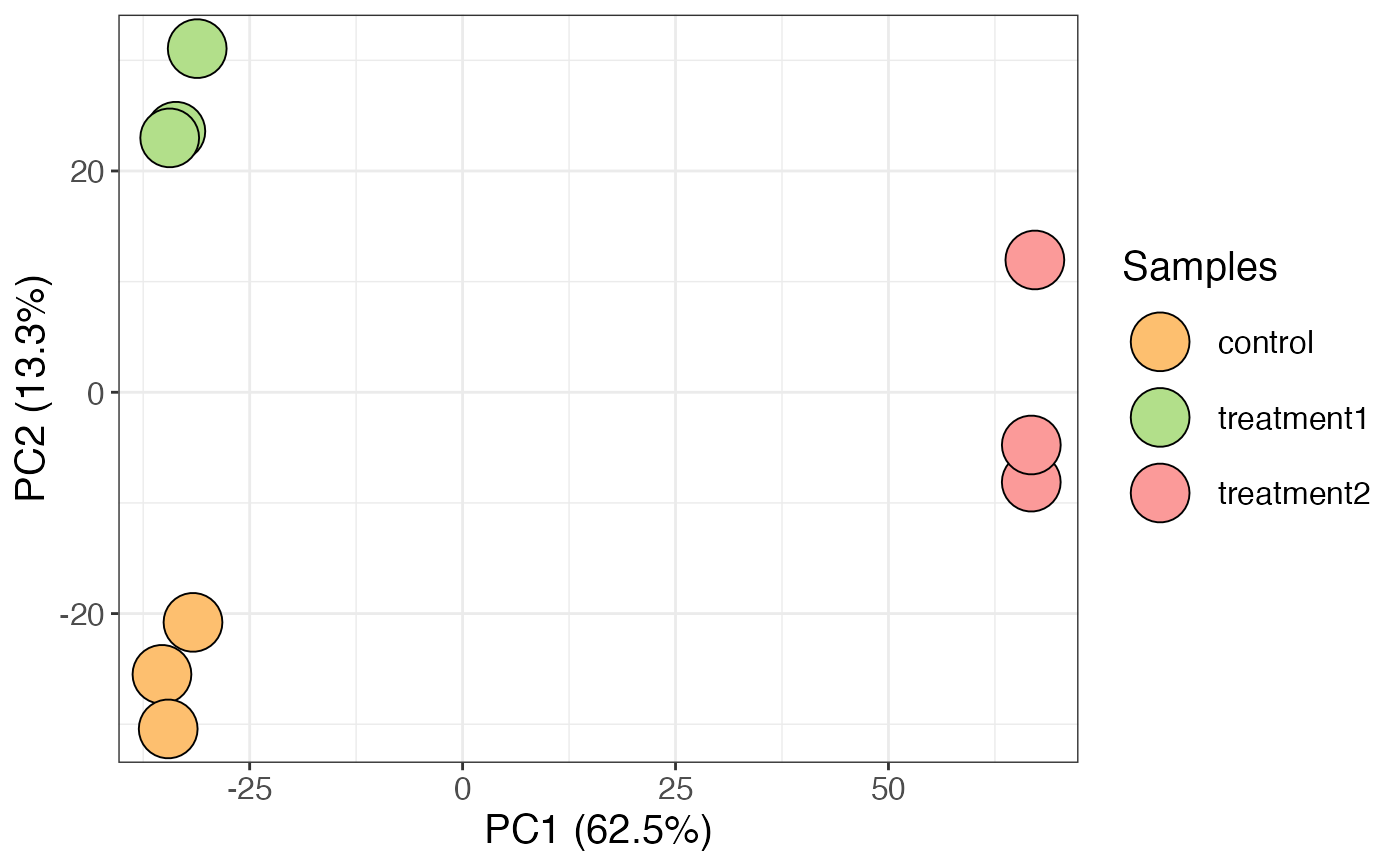
get_pca_plot(x = res,sample_colors = TRUE, sample.seed = 345) %>% print()
# reproduce sampled colors with argument `sample.seed`
get_pca_plot(x = res,sample_colors = TRUE, sample.seed = 345) %>% print()
 # label replicates
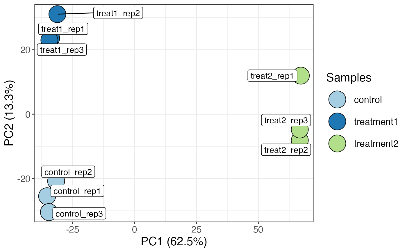
get_pca_plot(x = res, sample_colors = FALSE,label_replicates = TRUE)
# label replicates
get_pca_plot(x = res, sample_colors = FALSE,label_replicates = TRUE)