Generate upset plots for differently expressed genes between comparisons.
Source:R/rnaseq_related.R
plot_deg_upsets.RdFor a given set of DEG comparisons, the functions returns UpSetR::upset() plots for up and down genes between any 2 comparisons.
For each upset plot generated function also returns interaction between gene sets in form of dataframe.
Arguments
- x
x an abject of class "parcutils". This is an output of the function
run_deseq_analysis().- sample_comparisons
a character vector denoting sample comparisons between upset plot to be generated.
- color_up
a character string denoting a valid color code for bars in upset plot for up regulated genes.
- color_down
a character string denoting a valid color code for bars in upset plot for down regulated genes.
Value
an object of named list where each element is a list of two - 1) an upset plots UpSetR::upset() and their intersections in form of tibble.
Examples
count_file <- system.file("extdata","toy_counts.txt" , package = "parcutils")
count_data <- readr::read_delim(count_file, delim = "\t")
#> Rows: 5000 Columns: 10
#> ── Column specification ────────────────────────────────────────────────────────
#> Delimiter: "\t"
#> chr (1): gene_id
#> dbl (9): control_rep1, control_rep2, control_rep3, treat1_rep1, treat1_rep2,...
#>
#> ℹ Use `spec()` to retrieve the full column specification for this data.
#> ℹ Specify the column types or set `show_col_types = FALSE` to quiet this message.
sample_info <- count_data %>% colnames() %>% .[-1] %>%
tibble::tibble(samples = . , groups = rep(c("control" ,"treatment1" , "treatment2"), each = 3) )
res <- run_deseq_analysis(counts = count_data ,
sample_info = sample_info,
column_geneid = "gene_id" ,
group_numerator = c("treatment1", "treatment2") ,
group_denominator = c("control"))
#> ℹ Running DESeq2 ...
#> converting counts to integer mode
#> Warning: some variables in design formula are characters, converting to factors
#> estimating size factors
#> estimating dispersions
#> gene-wise dispersion estimates
#> mean-dispersion relationship
#> final dispersion estimates
#> fitting model and testing
#> ✔ Done.
#> ℹ Summarizing DEG ...
#> ✔ Done.
yy <- plot_deg_upsets(x= res, sample_comparisons = c("treatment1_VS_control","treatment2_VS_control"))
yy[[1]]$upset_plot %>% print()
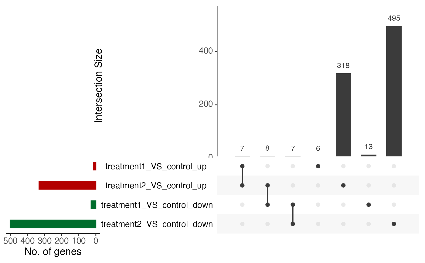 yy[[1]]$upset_intersects %>% print()
#> # A tibble: 7 × 2
#> set elements
#> <chr> <list>
#> 1 treatment1_VS_control_up <chr [6]>
#> 2 treatment1_VS_control_up,treatment2_VS_control_up <chr [7]>
#> 3 treatment2_VS_control_up <chr [318]>
#> 4 treatment2_VS_control_up,treatment1_VS_control_down <chr [8]>
#> 5 treatment1_VS_control_down,treatment2_VS_control_down <chr [7]>
#> 6 treatment1_VS_control_down <chr [13]>
#> 7 treatment2_VS_control_down <chr [495]>
yy[[1]]$upset_intersects %>% print()
#> # A tibble: 7 × 2
#> set elements
#> <chr> <list>
#> 1 treatment1_VS_control_up <chr [6]>
#> 2 treatment1_VS_control_up,treatment2_VS_control_up <chr [7]>
#> 3 treatment2_VS_control_up <chr [318]>
#> 4 treatment2_VS_control_up,treatment1_VS_control_down <chr [8]>
#> 5 treatment1_VS_control_down,treatment2_VS_control_down <chr [7]>
#> 6 treatment1_VS_control_down <chr [13]>
#> 7 treatment2_VS_control_down <chr [495]>