
Raincloud Plots in VISTA
VISTA Development Team
Source:vignettes/guides/VISTA-raincloud.Rmd
VISTA-raincloud.RmdOverview
Raincloud plots combine three visual layers:
- distribution shape (half-violin),
- robust summary (boxplot), and
- individual observations (jittered points).
This vignette shows raincloud plotting for both expression and
fold-change data in VISTA, including line-connection control with
id.long.var and optional statistical annotations.
Create a VISTA object
library(VISTA)
library(ggplot2)

data("count_data", package = "VISTA")
data("sample_metadata", package = "VISTA")

# Keep runtime modest for vignette rendering
count_small <- count_data[1:1000, ]

vista <- create_vista(
  counts = count_small,
  sample_info = sample_metadata,
  column_geneid = "gene_id",
  group_column = "cond_long",
  group_numerator = "treatment1",
  group_denominator = "control",
  method = "deseq2",
  min_counts = 10,
  min_replicates = 1
)

comp_names <- names(comparisons(vista))
top_up <- get_genes_by_regulation(
  vista,
  sample_comparisons = comp_names[1],
  regulation = "Up"
)
n_select_genes = 50
selected_genes <- stats::na.omit(utils::head(top_up$gene_id, n_select_genes))
if (!length(selected_genes)) {
  selected_genes <- rownames(vista)[1:n_select_genes]
}
Expression Raincloud
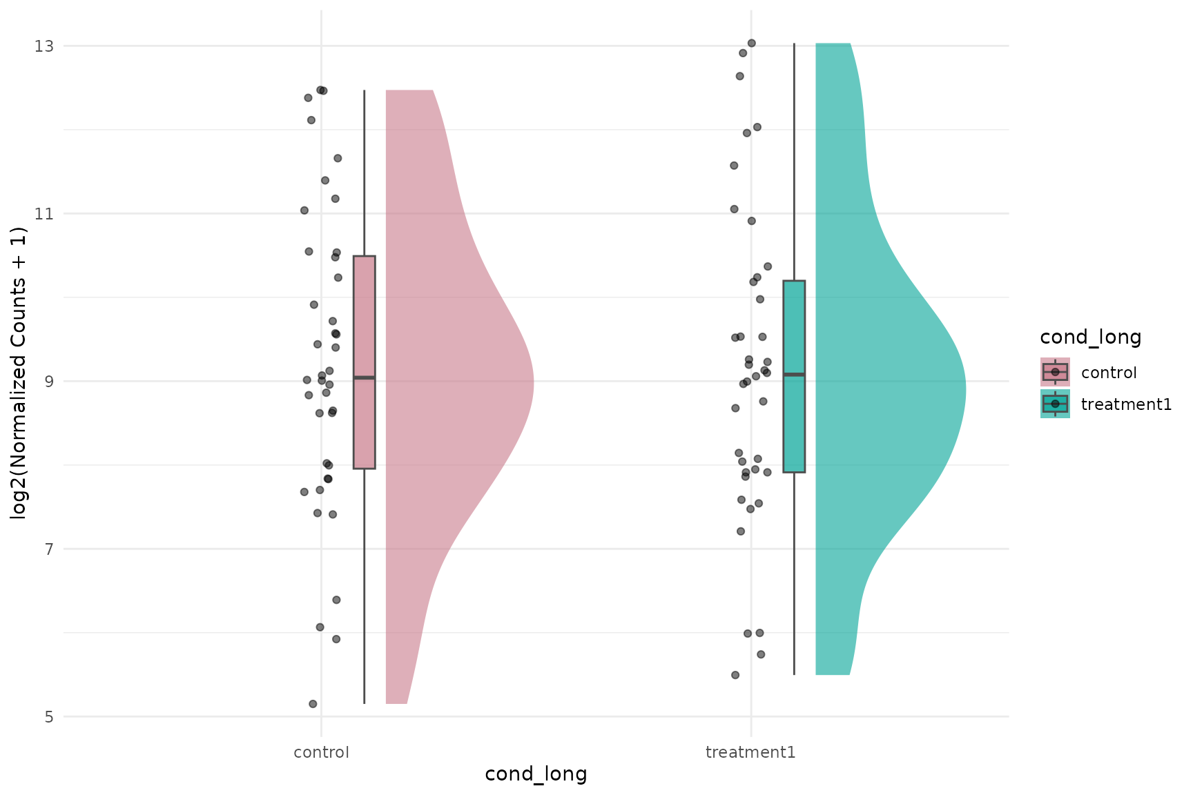
Basic expression raincloud (pooled gene-sample values)
get_expression_raincloud(
  vista,
  genes = selected_genes[1:10],
  value_transform = "log2",
  summarise = FALSE,
  facet_by = "none"
)
summarise = FALSE vs summarise = TRUE
For expression rainclouds:
-
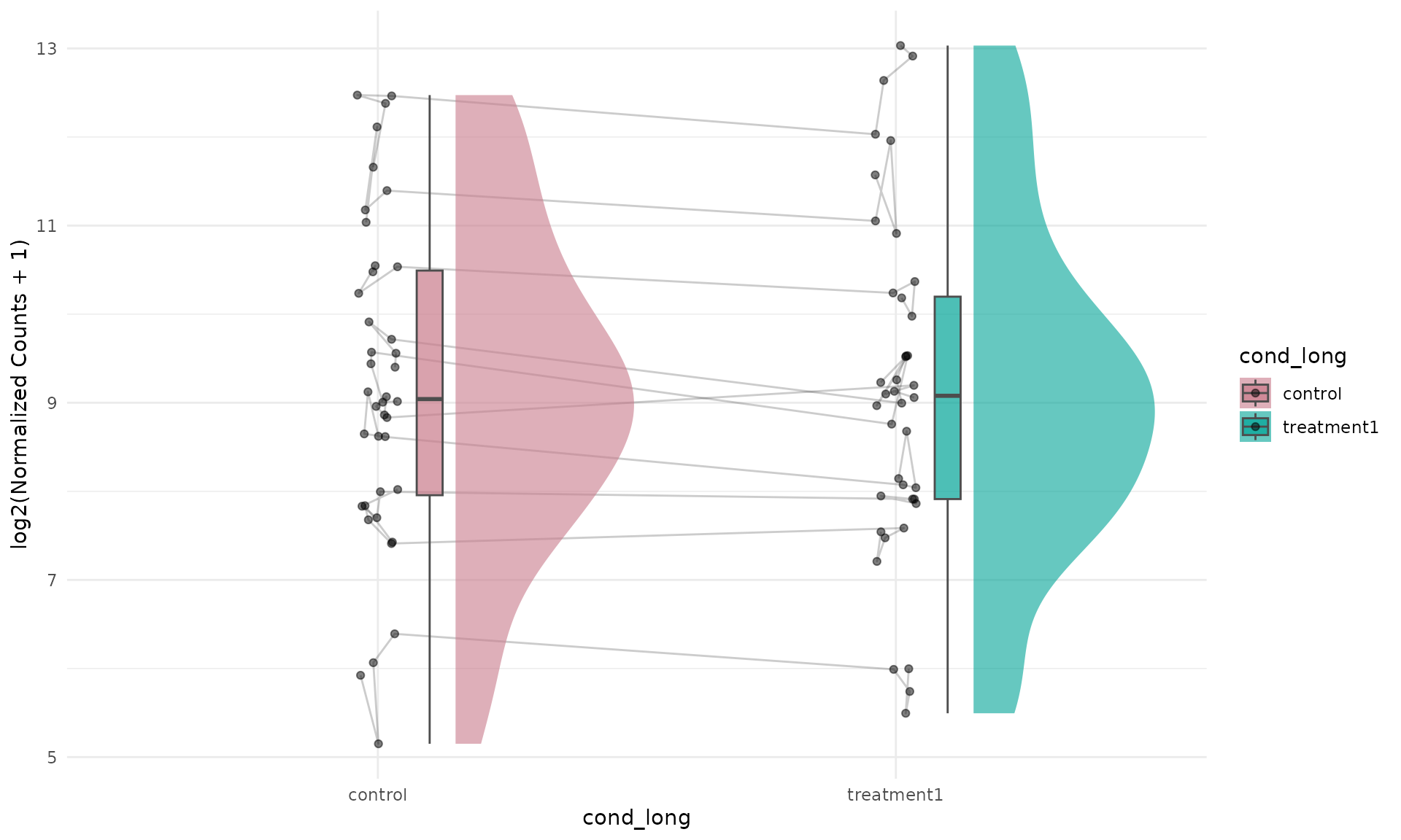
summarise = FALSE: each point is a gene-sample value (pooled across selected genes). -
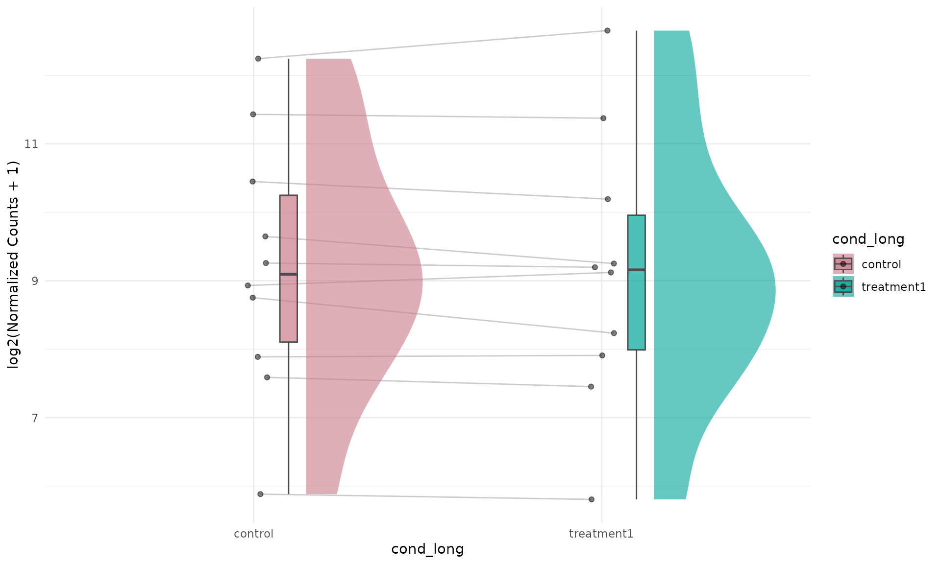
summarise = TRUE: each point is a gene-level group summary (one value per gene per group).
With summarise = TRUE, using
id.long.var = "gene" is useful for connecting each gene
across groups.
get_expression_raincloud(
  vista,
  genes = selected_genes[1:10],
  value_transform = "log2",
  summarise = FALSE,
  facet_by = "none",
  id.long.var = "gene"
)
get_expression_raincloud(
  vista,
  genes = selected_genes[1:10],
  value_transform = "log2",
  summarise = TRUE,
  facet_by = "none",
  id.long.var = "gene"
)
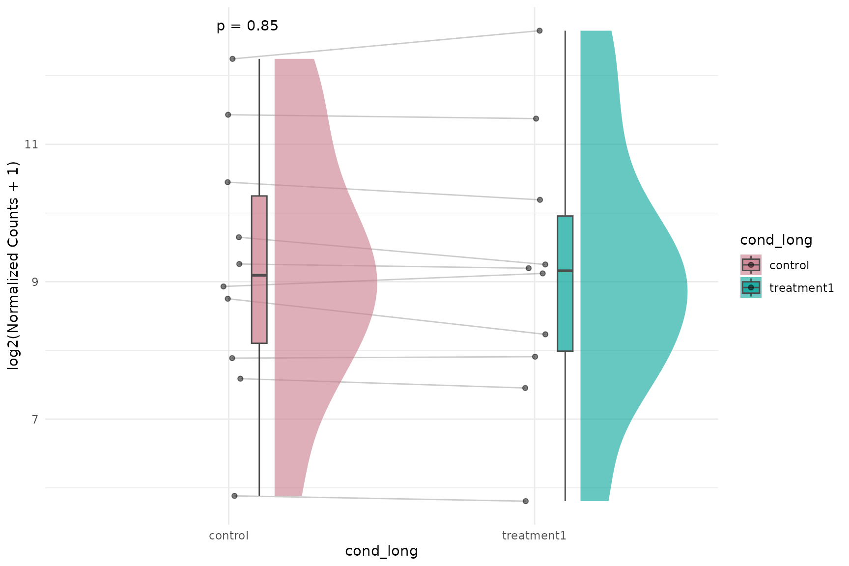
Expression raincloud with lines and p-values
get_expression_raincloud(
  vista,
  genes = selected_genes[1:10],
  value_transform = "log2",
  summarise = TRUE,
  facet_by = "none",
  id.long.var = "gene",
  stats_group = TRUE,
  stats_method = "wilcox.test",
  p.label = "p.format"
)
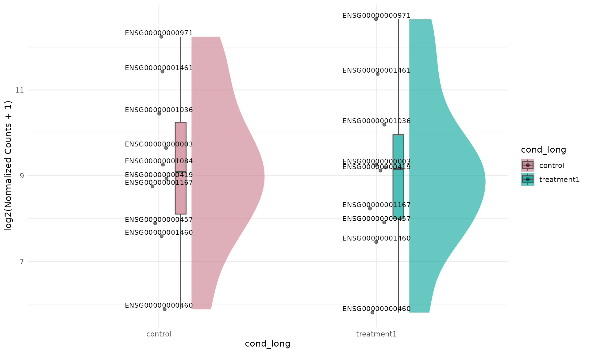
Label dots by gene ID (facet_by = "none")
get_expression_raincloud(
  vista,
  genes = selected_genes[1:10],
  value_transform = "log2",
  summarise = TRUE,
  facet_by = "none",
  label = TRUE,
  label_column = "gene",
  label_size = 3
)
If your object has symbol annotations in rowData(vista)
(or you provide display_from/display_orgdb),
you can label directly in symbol space:
get_expression_raincloud(
  vista,
  genes = c("NFKBIA", "KLF6", "PER1"),
  value_transform = "log2",
  summarise = TRUE,
  facet_by = "none",
  label = TRUE,
  display_id = "SYMBOL"
)
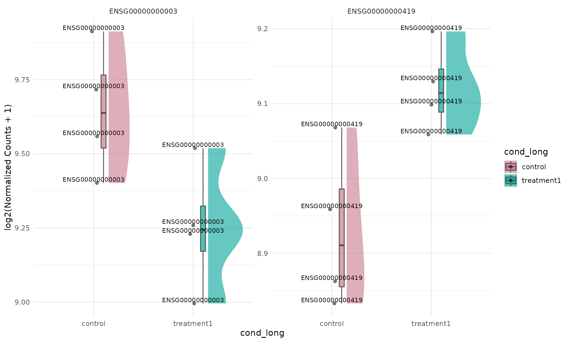
When facet_by = "gene", prefer
summarise = FALSE so each facet retains replicate-level
distribution. With summarise = TRUE, each facet has only
group-level summaries and the raincloud shape is usually not
informative.
get_expression_raincloud(
  vista,
  genes = selected_genes[1:2],
  value_transform = "log2",
  summarise = FALSE,
  facet_by = "gene",
  label = TRUE,
  label_column = "gene",
  label_size = 2.8
)
Flipped expression raincloud
Raincloud plots can be visually emphasized in a horizontal layout by
combining a left-side raincloud with coord_flip().
get_expression_raincloud(
  vista,
  genes = selected_genes[1:10],
  value_transform = "log2",
  summarise = TRUE,
  facet_by = "none",
  rain_side = "r",
  id.long.var = "gene"
) +
  ggplot2::coord_flip()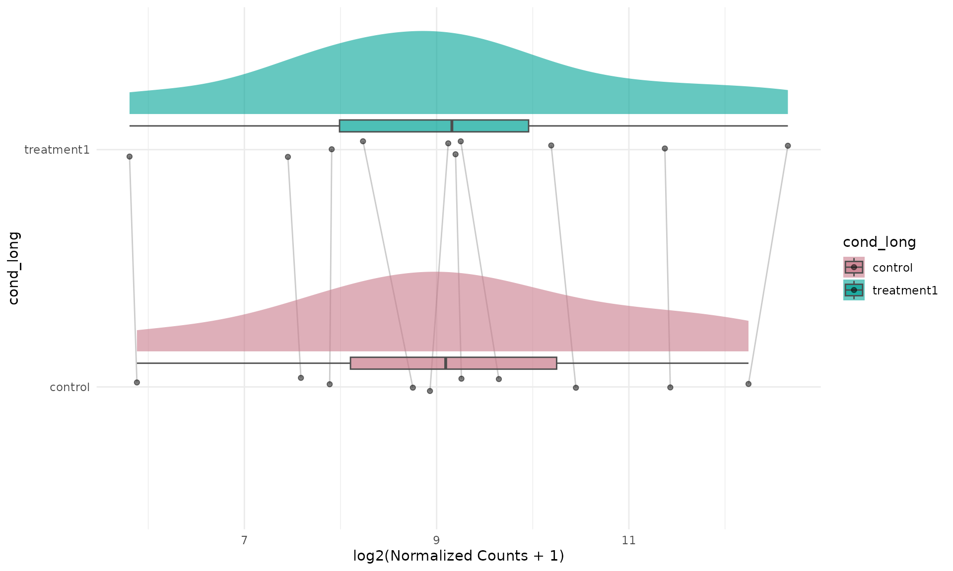
Fold-Change Raincloud
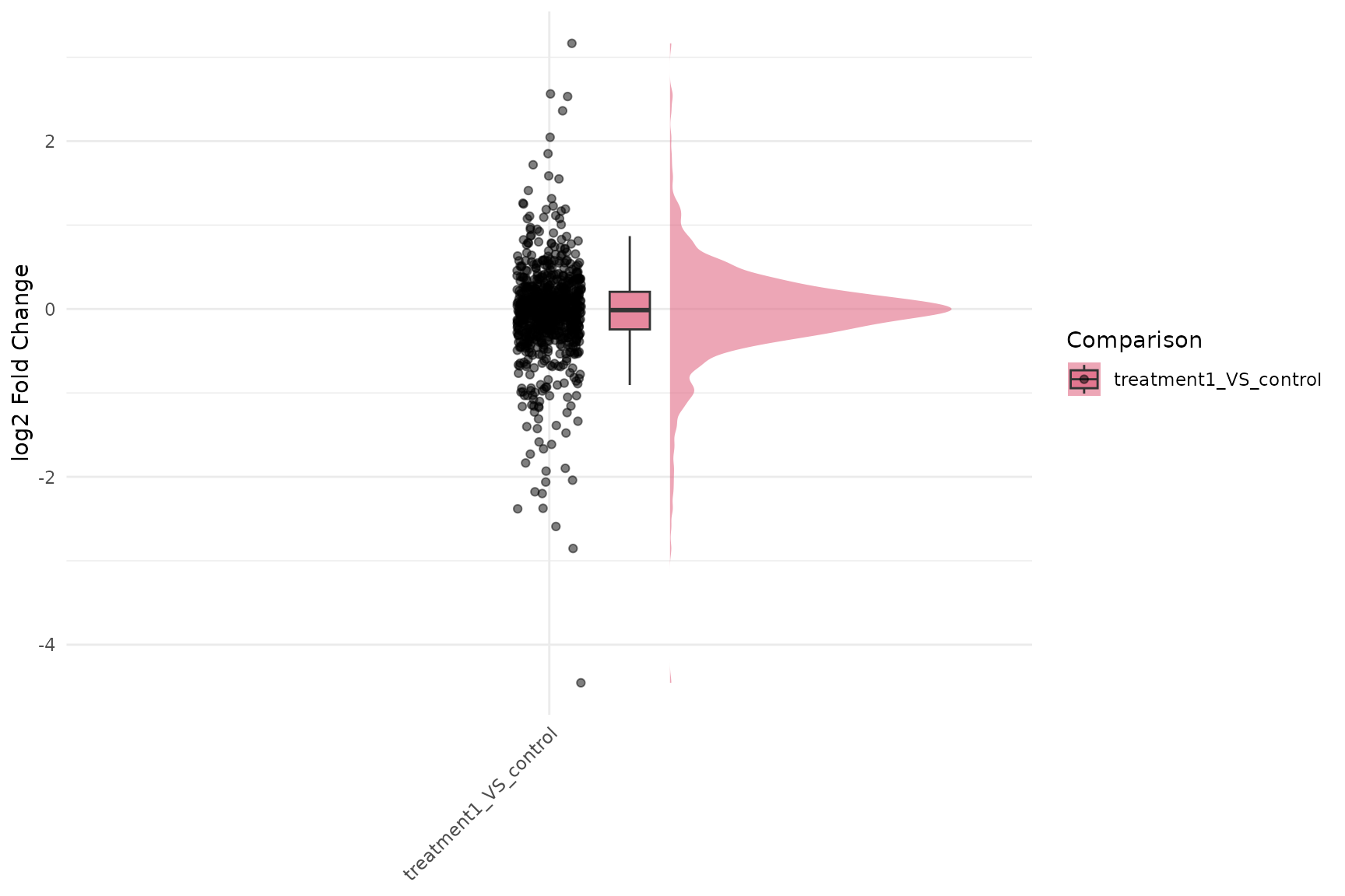
Basic fold-change raincloud
get_foldchange_raincloud(
  vista,
  sample_comparisons = comp_names,
  facet_by = "auto"
)
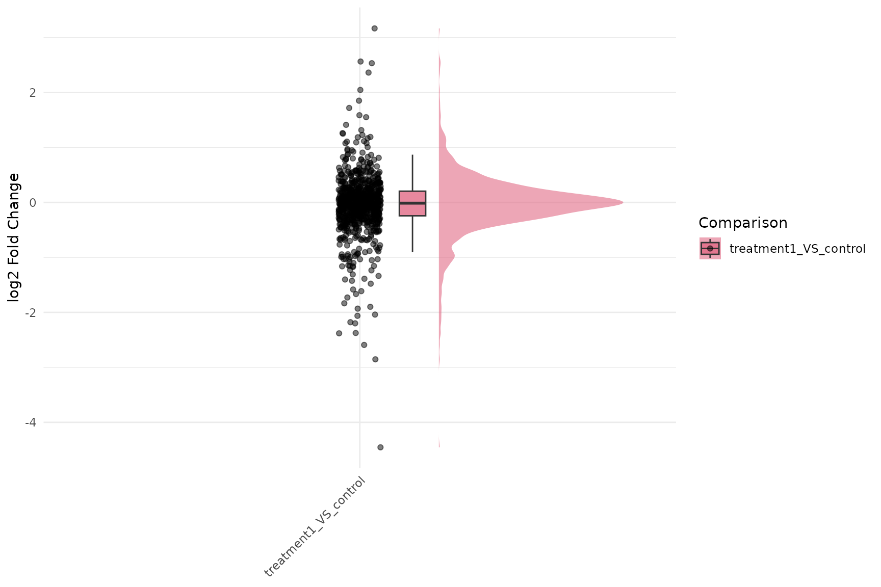
Fold-change raincloud with gene trajectories and p-values
get_foldchange_raincloud(
  vista,
  sample_comparisons = comp_names,
  facet_by = "none",
  id.long.var = "gene_id",
  stats_group = TRUE,
  stats_method = "t.test"
)
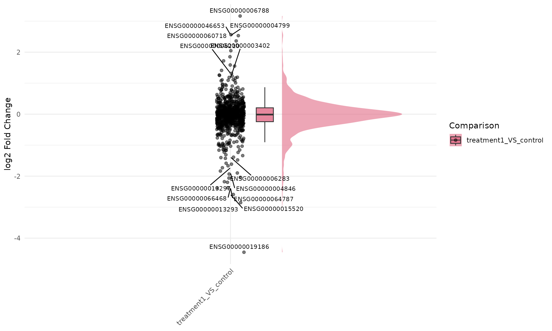
Label dots by gene ID for fold-change raincloud
get_foldchange_raincloud(
  vista,
  sample_comparisons = comp_names,
  facet_by = "none",
  label = TRUE,
  label_column = "gene_id",
  label_size = 2.8
)
get_foldchange_raincloud(
  vista,
  genes = c("NFKBIA", "KLF6", "PER1"),
  sample_comparisons = comp_names,
  facet_by = "none",
  label = TRUE,
  display_id = "SYMBOL"
)
Flipped fold-change raincloud
get_foldchange_raincloud(
  vista,
  sample_comparisons = comp_names,
  facet_by = "none",
  rain_side = "r",
  id.long.var = "gene_id"
) +
  ggplot2::coord_flip()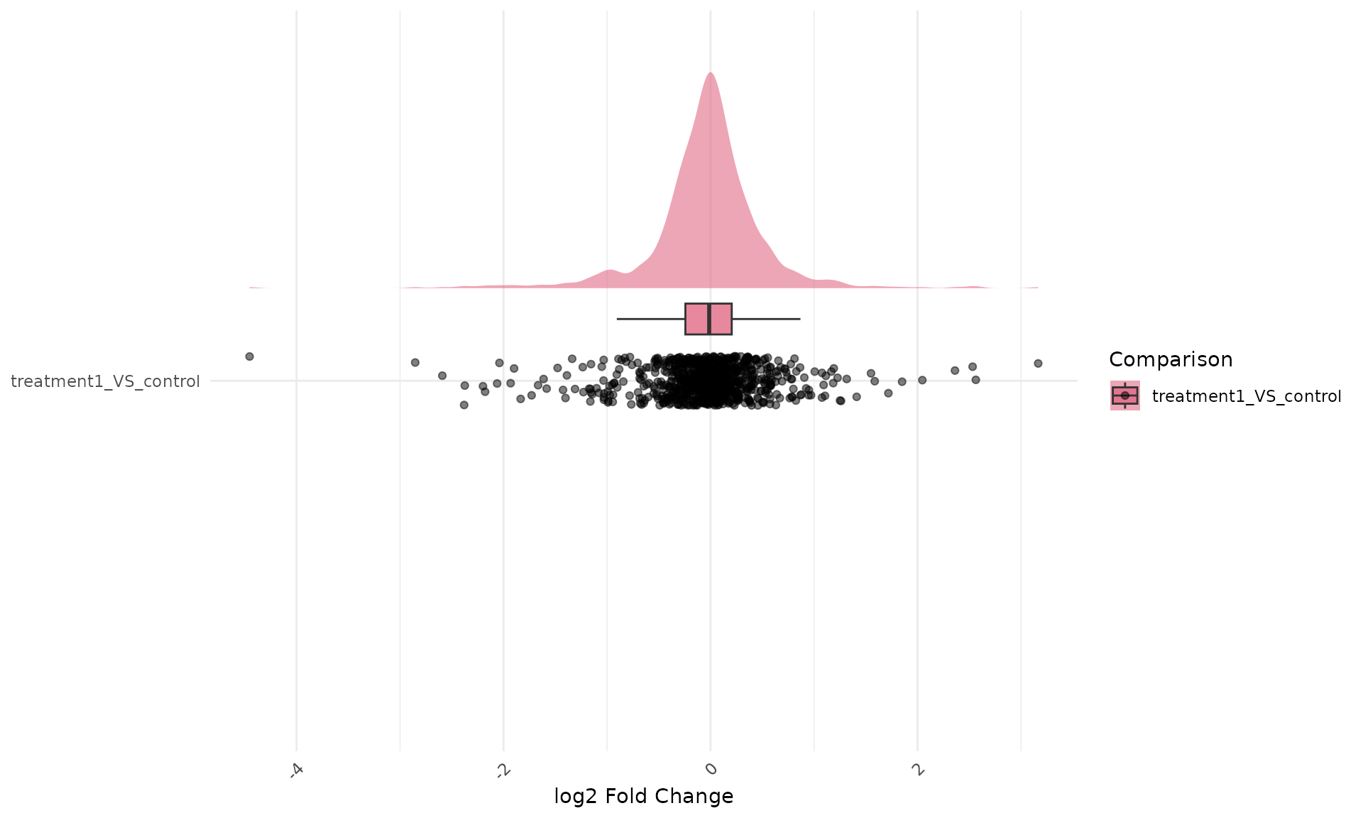
Why this is harder outside VISTA
Outside VISTA, producing equivalent raincloud plots is more involved because you must manually:
- extract and harmonize DE tables per comparison,
- reshape to long format for plotting,
- track grouping and palette consistency,
- map repeated-measure identifiers for line connections, and
- add and control statistical annotations per plotting context.
A minimal non-VISTA workflow typically requires custom wrangling and multiple plot-specific settings:
# 1) Build long expression/fold-change tables manually
# 2) Join sample metadata and comparison metadata
# 3) Validate IDs for repeated measures (id.long.var)
# 4) Create raincloud layers and palette mapping
# 5) Add statistical comparisons and label formatting
# 6) Repeat the process for each analysis object/comparison set
In VISTA, these steps are encapsulated in
get_expression_raincloud() and
get_foldchange_raincloud() while staying consistent with
the rest of the plotting API.
Session information
sessionInfo()
#> R version 4.6.1 (2026-06-24)
#> Platform: x86_64-pc-linux-gnu
#> Running under: Ubuntu 24.04.5 LTS
#>
#> Matrix products: default
#> BLAS:   /usr/lib/x86_64-linux-gnu/openblas-pthread/libblas.so.3
#> LAPACK: /usr/lib/x86_64-linux-gnu/openblas-pthread/libopenblasp-r0.3.26.so;  LAPACK version 3.12.0
#>
#> locale:
#>  [1] LC_CTYPE=C.UTF-8       LC_NUMERIC=C           LC_TIME=C.UTF-8
#>  [4] LC_COLLATE=C.UTF-8     LC_MONETARY=C.UTF-8    LC_MESSAGES=C.UTF-8
#>  [7] LC_PAPER=C.UTF-8       LC_NAME=C              LC_ADDRESS=C
#> [10] LC_TELEPHONE=C         LC_MEASUREMENT=C.UTF-8 LC_IDENTIFICATION=C
#>
#> time zone: UTC
#> tzcode source: system (glibc)
#>
#> attached base packages:
#> [1] stats     graphics  grDevices utils     datasets  methods   base
#>
#> other attached packages:
#> [1] ggplot2_4.0.3    VISTA_1.1.7      BiocStyle_2.40.0
#>
#> loaded via a namespace (and not attached):
#>   [1] RColorBrewer_1.1-3          ggrain_0.1.2
#>   [3] jsonlite_2.0.0              tidydr_0.0.7
#>   [5] magrittr_2.0.5              ggtangle_0.1.4
#>   [7] farver_2.1.2                rmarkdown_2.32
#>   [9] fs_2.1.0                    ragg_1.5.2
#>  [11] vctrs_0.7.3                 memoise_2.0.1
#>  [13] ggtree_4.2.0                rstatix_1.1.0
#>  [15] htmltools_0.5.9             S4Arrays_1.12.1
#>  [17] polynom_1.4-1               broom_1.0.13
#>  [19] Formula_1.2-6               SparseArray_1.12.3
#>  [21] gridGraphics_0.5-1          sass_0.4.10
#>  [23] bslib_0.12.0                htmlwidgets_1.6.4
#>  [25] desc_1.4.3                  plyr_1.8.9
#>  [27] httr2_1.3.0                 cachem_1.1.0
#>  [29] igraph_2.3.4                lifecycle_1.0.5
#>  [31] pkgconfig_2.0.3             gson_0.2.2
#>  [33] Matrix_1.7-5                R6_2.6.1
#>  [35] fastmap_1.2.0               MatrixGenerics_1.24.0
#>  [37] digest_0.6.39               aplot_0.3.2
#>  [39] enrichplot_1.32.1           colorspace_2.1-4
#>  [41] ggnewscale_0.5.2            GGally_2.4.0
#>  [43] patchwork_1.3.2             AnnotationDbi_1.74.0
#>  [45] S4Vectors_0.50.3            aisdk_1.4.12
#>  [47] ps_1.9.3                    DESeq2_1.52.0
#>  [49] textshaping_1.0.5           GenomicRanges_1.64.0
#>  [51] RSQLite_3.53.3              ggpubr_1.0.0
#>  [53] labeling_0.4.3              polyclip_1.10-7
#>  [55] httr_1.4.9                  abind_1.4-8
#>  [57] compiler_4.6.1              withr_3.0.3
#>  [59] bit64_4.8.6                 fontquiver_0.2.1
#>  [61] backports_1.5.1             S7_0.2.2
#>  [63] BiocParallel_1.46.0         carData_3.0-6
#>  [65] DBI_1.3.0                   ggstats_0.14.0
#>  [67] ggforce_0.5.0               ggsignif_0.6.4
#>  [69] MASS_7.3-65                 rappdirs_0.3.4
#>  [71] DelayedArray_0.38.2         ggpp_0.6.1
#>  [73] tools_4.6.1                 otel_0.2.0
#>  [75] scatterpie_0.2.6            ape_5.8-1
#>  [77] msigdbr_26.1.1              glue_1.8.1
#>  [79] callr_3.8.0                 nlme_3.1-169
#>  [81] GOSemSim_2.38.3             grid_4.6.1
#>  [83] cluster_2.1.8.2             reshape2_1.4.5
#>  [85] generics_0.1.4              gtable_0.3.6
#>  [87] tidyr_1.3.2                 car_3.1-5
#>  [89] XVector_0.52.0              BiocGenerics_0.58.1
#>  [91] ggrepel_0.9.8               pillar_1.11.1
#>  [93] stringr_1.6.0               limma_3.68.5
#>  [95] yulab.utils_0.2.5           splines_4.6.1
#>  [97] tweenr_2.0.3                dplyr_1.2.1
#>  [99] treeio_1.36.1               lattice_0.22-9
#> [101] bit_4.6.0                   tidyselect_1.2.1
#> [103] fontLiberation_0.1.0        GO.db_3.23.1
#> [105] locfit_1.5-9.12             Biostrings_2.80.2
#> [107] knitr_1.52                  fontBitstreamVera_0.1.1
#> [109] bookdown_0.48               IRanges_2.46.0
#> [111] Seqinfo_1.2.0               edgeR_4.10.7
#> [113] SummarizedExperiment_1.42.0 stats4_4.6.1
#> [115] xfun_0.62                   Biobase_2.72.0
#> [117] statmod_1.5.2               matrixStats_1.5.0
#> [119] stringi_1.8.9               lazyeval_0.2.3
#> [121] ggfun_0.2.2                 yaml_2.3.12
#> [123] evaluate_1.0.5              codetools_0.2-20
#> [125] qvalue_2.44.0               gdtools_0.5.2
#> [127] tibble_3.3.1                BiocManager_1.30.27
#> [129] ggplotify_0.1.4             cli_3.6.6
#> [131] systemfonts_1.3.2           processx_3.9.0
#> [133] jquerylib_0.1.4             Rcpp_1.1.2
#> [135] png_0.1-9                   parallel_4.6.1
#> [137] assertthat_0.2.1            pkgdown_2.2.1
#> [139] blob_1.3.0                  clusterProfiler_4.20.3
#> [141] DOSE_4.6.0                  tidytree_0.4.8
#> [143] ggiraph_0.9.6               enrichit_0.2.6
#> [145] scales_1.4.0                purrr_1.2.2
#> [147] crayon_1.5.3                rlang_1.3.0
#> [149] KEGGREST_1.52.2