Complete RNA-seq Analysis Workflow with VISTA
VISTA Development Team
Source:vignettes/VISTA-airway.Rmd
VISTA-airway.RmdIntroduction
This vignette demonstrates a complete RNA-seq differential expression workflow using VISTA (Visualization and Integrated System for Transcriptomic Analysis). We’ll use the well-known airway dataset from Bioconductor, which contains RNA-seq data from airway smooth muscle cells treated with dexamethasone.
What is VISTA?
VISTA streamlines RNA-seq analysis by:
- Unifying DE workflows: Wraps DESeq2 and edgeR with consistent output
- Simplifying visualization: 28+ publication-ready plotting functions
- Integrating enrichment: Built-in MSigDB, GO, and KEGG analysis
- Ensuring reproducibility: S4 class structure with comprehensive metadata
Dataset Overview
The airway dataset (Himes et al. 2014) includes:
- Samples: 8 human airway smooth muscle cell lines
- Treatment: 4 treated with dexamethasone, 4 untreated
- Sequencing: Illumina HiSeq 2000
- Features: ~64,000 genes
Reference: Himes BE et al. (2014). “RNA-Seq transcriptome profiling identifies CRISPLD2 as a glucocorticoid responsive gene that modulates cytokine function in airway smooth muscle cells.” PLoS One 9(6): e99625.
Installation and Setup
if (!requireNamespace("BiocManager", quietly = TRUE)) {
  install.packages("BiocManager")
}

BiocManager::install(c("VISTA", "airway", "org.Hs.eg.db"))
install.packages("ggplot2")
# Load required packages
library(VISTA)
library(ggplot2)         # For plotting functions
library(airway)          # Dataset
library(org.Hs.eg.db)    # Human gene annotations
library(magrittr)    # %>%
If required packages are missing, install them before rendering this vignette.
Data Preparation
Load the airway dataset
# Load the SummarizedExperiment object
data("airway", package = "airway")

# Examine the structure
airway
#> class: RangedSummarizedExperiment
#> dim: 63677 8
#> metadata(1): ''
#> assays(1): counts
#> rownames(63677): ENSG00000000003 ENSG00000000005 ... ENSG00000273492
#>   ENSG00000273493
#> rowData names(10): gene_id gene_name ... seq_coord_system symbol
#> colnames(8): SRR1039508 SRR1039509 ... SRR1039520 SRR1039521
#> colData names(9): SampleName cell ... Sample BioSample
Extract counts and metadata
# Extract count matrix
counts_matrix <- assay(airway, "counts")

# Preview counts (first 5 genes, first 4 samples)
counts_matrix[1:5, 1:4]
#>                 SRR1039508 SRR1039509 SRR1039512 SRR1039513
#> ENSG00000000003        679        448        873        408
#> ENSG00000000005          0          0          0          0
#> ENSG00000000419        467        515        621        365
#> ENSG00000000457        260        211        263        164
#> ENSG00000000460         60         55         40         35

# Extract sample metadata
sample_metadata <- as.data.frame(colData(airway))
sample_metadata
#>            SampleName    cell   dex albut        Run avgLength Experiment
#> SRR1039508 GSM1275862  N61311 untrt untrt SRR1039508       126  SRX384345
#> SRR1039509 GSM1275863  N61311   trt untrt SRR1039509       126  SRX384346
#> SRR1039512 GSM1275866 N052611 untrt untrt SRR1039512       126  SRX384349
#> SRR1039513 GSM1275867 N052611   trt untrt SRR1039513        87  SRX384350
#> SRR1039516 GSM1275870 N080611 untrt untrt SRR1039516       120  SRX384353
#> SRR1039517 GSM1275871 N080611   trt untrt SRR1039517       126  SRX384354
#> SRR1039520 GSM1275874 N061011 untrt untrt SRR1039520       101  SRX384357
#> SRR1039521 GSM1275875 N061011   trt untrt SRR1039521        98  SRX384358
#>               Sample    BioSample
#> SRR1039508 SRS508568 SAMN02422669
#> SRR1039509 SRS508567 SAMN02422675
#> SRR1039512 SRS508571 SAMN02422678
#> SRR1039513 SRS508572 SAMN02422670
#> SRR1039516 SRS508575 SAMN02422682
#> SRR1039517 SRS508576 SAMN02422673
#> SRR1039520 SRS508579 SAMN02422683
#> SRR1039521 SRS508580 SAMN02422677

# Simplify treatment labels for clarity
sample_metadata$treatment <- ifelse(
  sample_metadata$dex == "trt",
  "Dexamethasone",
  "Untreated"
)
Prepare data for VISTA
VISTA includes helper functions that standardize counts and sample
metadata before calling create_vista():
prepared_counts <- read_vista_counts(
  counts_matrix,
  format = "matrix"
)

prepared_samples <- read_vista_metadata(
  sample_metadata %>%
    tibble::as_tibble() %>%
    dplyr::rename("sample_names" = "Run")
)

matched_inputs <- match_vista_inputs(prepared_counts, prepared_samples)

# Preview the create_vista-ready count table
matched_inputs$counts[1:5, 1:5]
#>                         gene_id SRR1039508 SRR1039509 SRR1039512 SRR1039513
#> ENSG00000000003 ENSG00000000003        679        448        873        408
#> ENSG00000000005 ENSG00000000005          0          0          0          0
#> ENSG00000000419 ENSG00000000419        467        515        621        365
#> ENSG00000000457 ENSG00000000457        260        211        263        164
#> ENSG00000000460 ENSG00000000460         60         55         40         35
For a more complete guide covering file-derived sample-name repair
and starter metadata generation with
derive_vista_metadata(), see the pkgdown article
Preparing Counts and Metadata for VISTA.
The matched sample sheet now has stable sample_names
aligned to the count columns:
matched_inputs$sample_info[, c("sample_names", "cell", "treatment", "dex")]
#>            sample_names    cell     treatment   dex
#> SRR1039508   SRR1039508  N61311     Untreated untrt
#> SRR1039509   SRR1039509  N61311 Dexamethasone   trt
#> SRR1039512   SRR1039512 N052611     Untreated untrt
#> SRR1039513   SRR1039513 N052611 Dexamethasone   trt
#> SRR1039516   SRR1039516 N080611     Untreated untrt
#> SRR1039517   SRR1039517 N080611 Dexamethasone   trt
#> SRR1039520   SRR1039520 N061011     Untreated untrt
#> SRR1039521   SRR1039521 N061011 Dexamethasone   trt
Create VISTA Object
Using DESeq2 backend
The primary method for creating a VISTA object:
# Create VISTA object with DESeq2 backend
vista <- create_vista(
  counts = matched_inputs$counts,
  sample_info = matched_inputs$sample_info,
  column_geneid = matched_inputs$column_geneid,
  group_column = "treatment",
  group_numerator = "Dexamethasone",
  group_denominator = "Untreated",
  method = "deseq2",
  min_counts = 10,
  min_replicates = 2,
  log2fc_cutoff = 1.0,
  pval_cutoff = 0.05,
  p_value_type = "padj"
)

# Examine the VISTA object
vista
#> class: VISTA
#> dim: 17199 8
#> metadata(12): de_results de_summary ... design comparison
#> assays(1): norm_counts
#> rownames(17199): ENSG00000000003 ENSG00000000419 ... ENSG00000273487
#>   ENSG00000273488
#> rowData names(1): baseMean
#> colnames(8): SRR1039508 SRR1039509 ... SRR1039520 SRR1039521
#> colData names(11): SampleName cell ... sizeFactor sample_names
The VISTA object stores:
-
Normalized counts in
assays -
Sample metadata in
colData -
Gene annotations in
rowData -
DE results in
metadata
Validate object integrity
create_vista() runs validation by default
(validate = TRUE). You can also run it explicitly:
validate_vista(vista, level = "full")For advanced users importing a pre-built
SummarizedExperiment, use as_vista() and then
validate:
se <- SummarizedExperiment::SummarizedExperiment(
  assays = list(norm_counts = norm_counts(vista)),
  colData = S4Vectors::DataFrame(sample_info(vista), row.names = sample_info(vista)$sample_names),
  rowData = S4Vectors::DataFrame(row_data(vista), row.names = rownames(norm_counts(vista)))
)
vista2 <- as_vista(se, group_column = "treatment")
validate_vista(vista2, level = "full")
Alternative: Using edgeR backend
# Create VISTA object with edgeR backend
vista_edger <- create_vista(
  counts = count_data,
  sample_info = sample_info,
  column_geneid = "gene_id",
  group_column = "treatment",
  group_numerator = "Dexamethasone",
  group_denominator = "Untreated",
  method = "edger",  # Use edgeR instead of DESeq2
  min_counts = 10,
  min_replicates = 2,
  log2fc_cutoff = 1.0,
  pval_cutoff = 0.05,
  p_value_type = "padj"
)
Alternative: Using limma-voom backend
# Create VISTA object with limma-voom backend
vista_limma <- create_vista(
  counts = count_data,
  sample_info = sample_info,
  column_geneid = "gene_id",
  group_column = "treatment",
  group_numerator = "Dexamethasone",
  group_denominator = "Untreated",
  method = "limma",
  min_counts = 10,
  min_replicates = 2,
  log2fc_cutoff = 1.0,
  pval_cutoff = 0.05,
  p_value_type = "padj"
)
Advanced: covariates, design formula, and consensus mode
# Covariate-adjusted model (additive design)
vista_cov <- create_vista(
  counts = count_data,
  sample_info = sample_info,
  column_geneid = "gene_id",
  group_column = "treatment",
  group_numerator = "Dexamethasone",
  group_denominator = "Untreated",
  method = "deseq2",
  covariates = c("cell")
)

# Equivalent explicit model formula
vista_formula <- create_vista(
  counts = count_data,
  sample_info = sample_info,
  column_geneid = "gene_id",
  group_column = "treatment",
  group_numerator = "Dexamethasone",
  group_denominator = "Untreated",
  method = "deseq2",
  design_formula = "~ cell + treatment"
)

# Run both DESeq2 and edgeR and keep consensus as active source
vista_both <- create_vista(
  counts = count_data,
  sample_info = sample_info,
  column_geneid = "gene_id",
  group_column = "treatment",
  group_numerator = "Dexamethasone",
  group_denominator = "Untreated",
  method = "both",
  consensus_mode = "intersection",  # or "union"
  result_source = "consensus"       # or "deseq2"/"edger"
)

# Access source-specific outputs
comparisons(vista_both, source = "consensus")
comparisons(vista_both, source = "deseq2")
comparisons(vista_both, source = "edger")

# Switch the active source used by plotting functions
vista_both <- set_de_source(vista_both, "edger")
Add gene annotations
Enhance the object with gene symbols and descriptions:
vista <- set_rowdata(
  vista,
  orgdb = org.Hs.eg.db,
  columns = c("SYMBOL", "GENENAME", "ENTREZID"),
  keytype = "ENSEMBL"
)

# View updated gene annotations
head(rowData(vista))
#> DataFrame with 6 rows and 4 columns
#>                  baseMean      SYMBOL               GENENAME    ENTREZID
#>                 <numeric> <character>            <character> <character>
#> ENSG00000000003  709.7752      TSPAN6          tetraspanin 6        7105
#> ENSG00000000419  521.1362        DPM1 dolichyl-phosphate m..        8813
#> ENSG00000000457  237.5619       SCYL3 SCY1 like pseudokina..       57147
#> ENSG00000000460   58.0338       FIRRM FIGNL1 interacting r..       55732
#> ENSG00000000971 5826.6231         CFH    complement factor H        3075
#> ENSG00000001036 1284.4108       FUCA2   alpha-L-fucosidase 2        2519
Explore the Results
Access differential expression results
# Get comparison names
comp_names <- names(comparisons(vista))
comp_names
#> [1] "Dexamethasone_VS_Untreated"
# Get DE results for the comparison
de_results <- comparisons(vista)[[1]]
head(de_results)
#> gene_id baseMean log2fc lfcSE stat
#> ENSG00000000003 ENSG00000000003 709.77518 -0.38027500 0.17108885 -2.2226756
#> ENSG00000000419 ENSG00000000419 521.13616 0.20227695 0.09533472 2.1217555
#> ENSG00000000457 ENSG00000000457 237.56187 0.03272066 0.12278673 0.2664837
#> ENSG00000000460 ENSG00000000460 58.03383 -0.11851609 0.30815777 -0.3845955
#> ENSG00000000971 ENSG00000000971 5826.62312 0.43942357 0.25944519 1.6937048
#> ENSG00000001036 ENSG00000001036 1284.41081 -0.24322719 0.11682555 -2.0819691
#> pvalue padj regulation
#> ENSG00000000003 0.02623769 0.1206592 Other
#> ENSG00000000419 0.03385828 0.1448222 Other
#> ENSG00000000457 0.78986672 0.9229371 Other
#> ENSG00000000460 0.70053714 0.8844114 Other
#> ENSG00000000971 0.09032139 0.2843077 Other
#> ENSG00000001036 0.03734529 0.1541257 Other
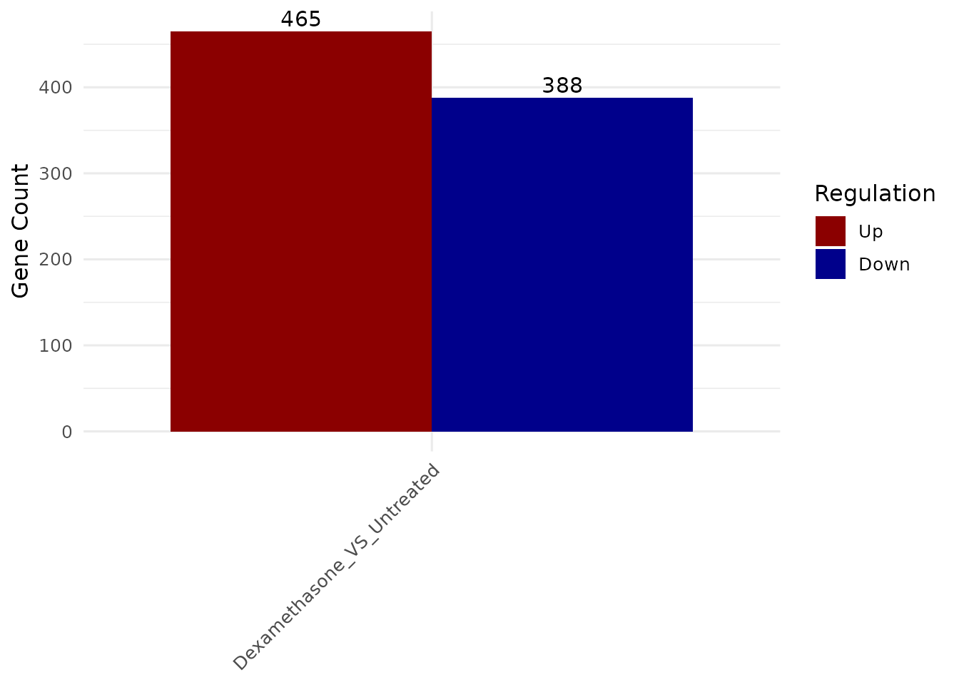
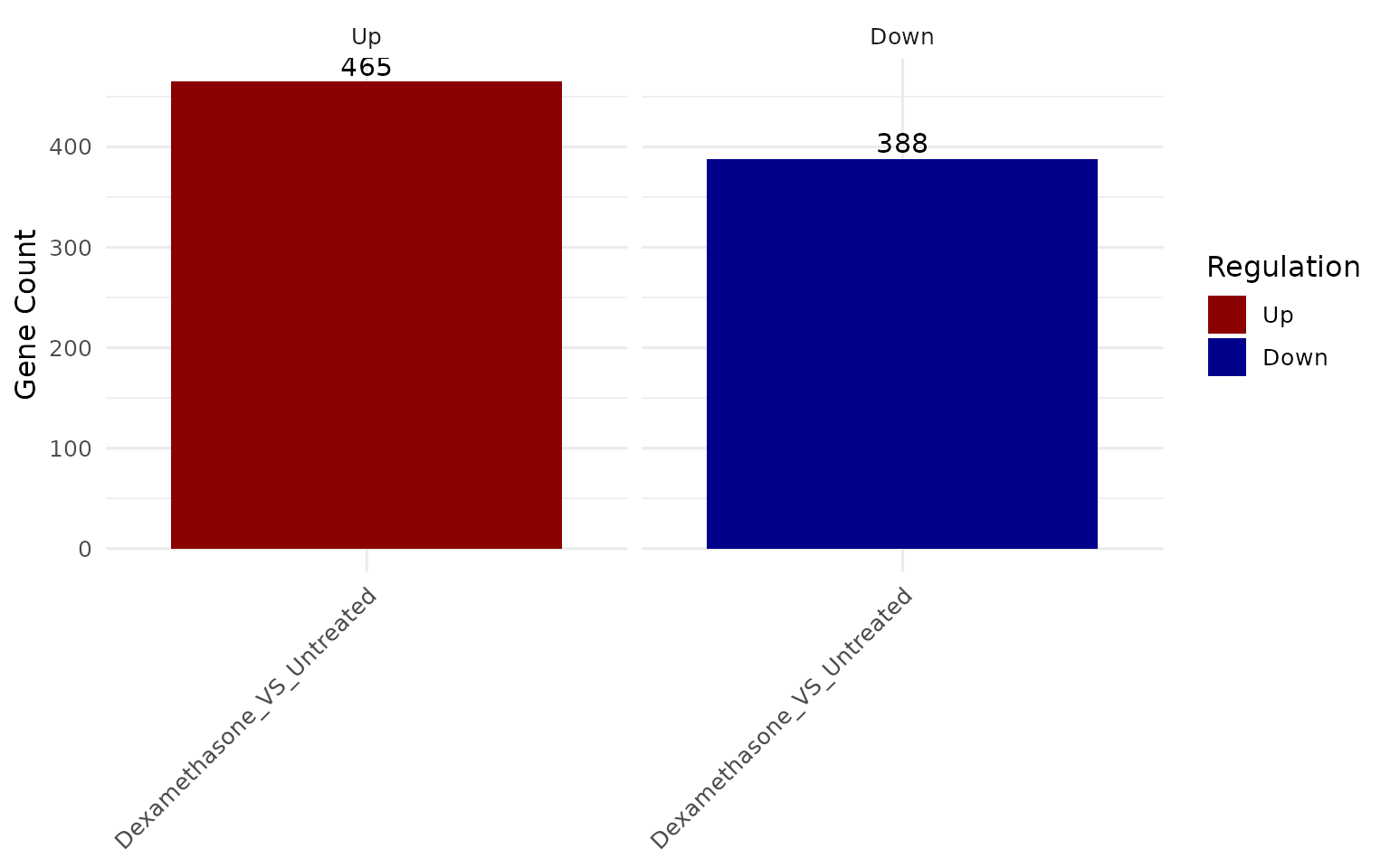
# Get DEG summary
deg_summary(vista)
#> $Dexamethasone_VS_Untreated
#> regulation n
#> 1 Down 388
#> 2 Other 16346
#> 3 Up 465
# Get analysis cutoffs
cutoffs(vista)
#> $log2fc
#> [1] 1
#>
#> $pval
#> [1] 0.05
#>
#> $p_value_type
#> [1] "padj"
#>
#> $method
#> [1] "deseq2"
#>
#> $min_counts
#> [1] 10
#>
#> $min_replicates
#> [1] 2
#>
#> $covariates
#> character(0)
#>
#> $design_formula
#> NULL
#>
#> $consensus_mode
#> NULL
#>
#> $consensus_log2fc
#> NULL
#>
#> $active_source
#> [1] "deseq2"Count significant genes
# Extract upregulated genes
up_genes <- get_genes_by_regulation(
  vista,
  sample_comparisons = comp_names[1],
  regulation = "Up",
  #top_n = 50
)

# Extract downregulated genes
down_genes <- get_genes_by_regulation(
  vista,
  sample_comparisons = comp_names[1],
  regulation = "Down",
  #top_n = 50
)

# Summary
cat("Upregulated genes:", length(up_genes[[1]]), "\n")
#> Upregulated genes: 465
cat("Downregulated genes:", length(down_genes[[1]]), "\n")
#> Downregulated genes: 388
Quality Control Visualizations
Sample Correlation Heatmap
Check sample relationships and potential batch effects.
Basic correlation heatmap
get_corr_heatmap(vista, label_size = 18,base_size = 18, viridis_direction = -1)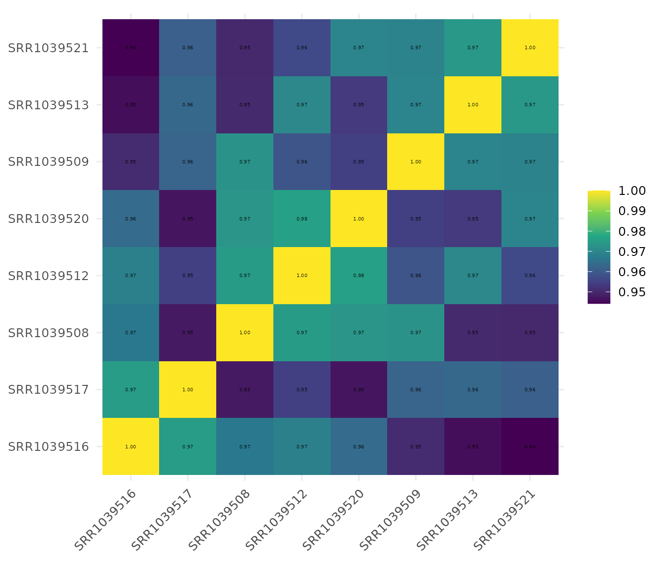
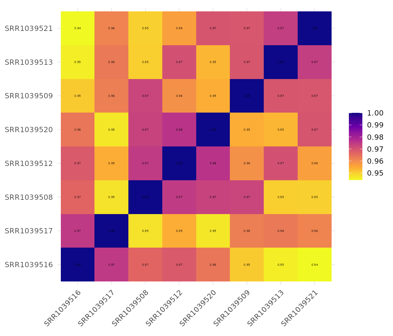
Customize color scheme
# Reverse viridis color direction
get_corr_heatmap(
  vista,
  viridis_direction = -1,
  viridis_option = "plasma",
  label_size = 18,
  base_size = 18
)
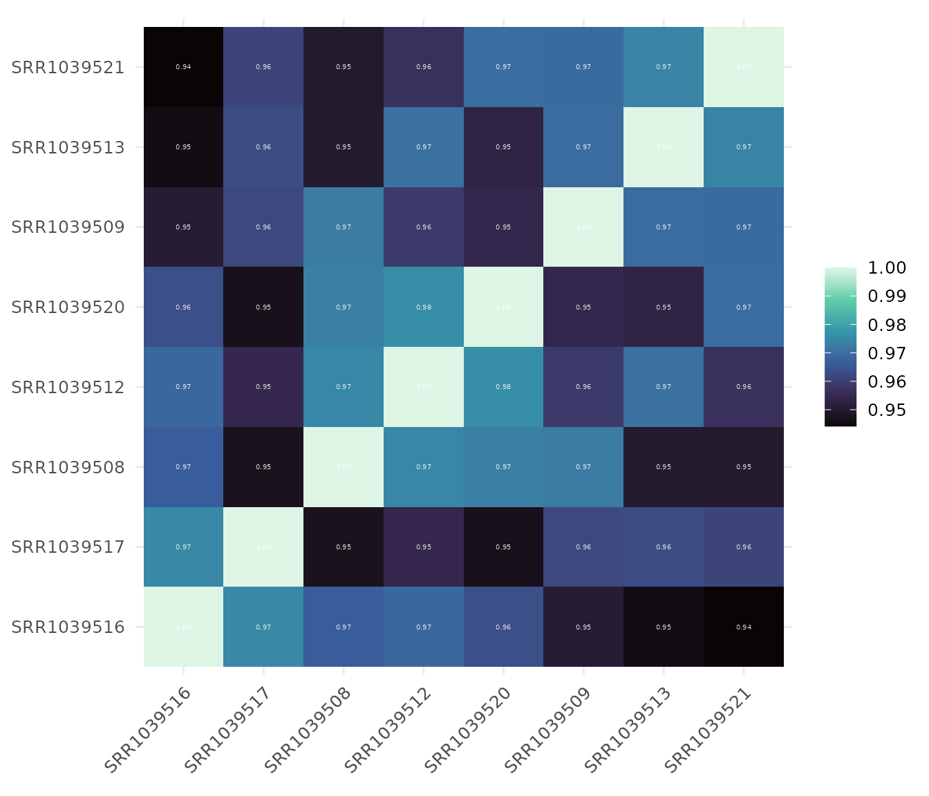
Show correlation values
# Display correlation coefficients
get_corr_heatmap(
  vista,
  viridis_direction = -1,
  show_corr_values = TRUE,
  col_corr_values = 'white',
  viridis_option = "mako",
  label_size = 14,
  base_size = 14
) 
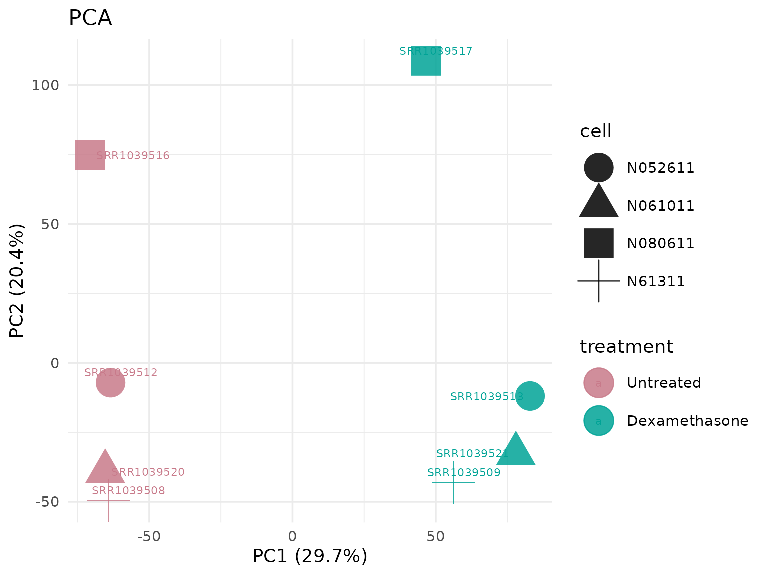
Principal Component Analysis (PCA)
Visualize sample clustering and variation.
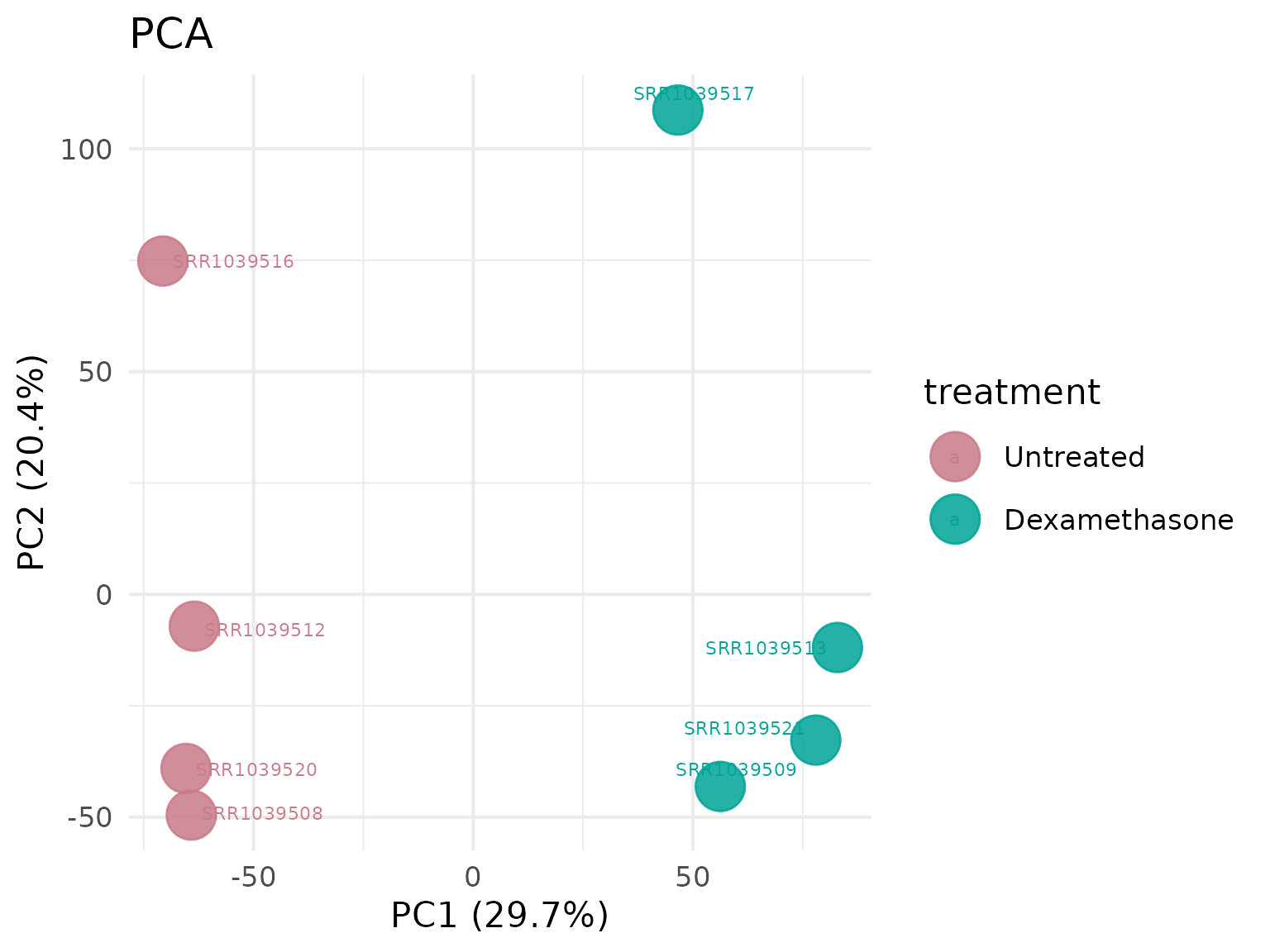
PCA colored by different metadata
# Shape points by cell line
get_pca_plot(
  vista,
  label = TRUE,
  label_size = 5,
  shape_by = "cell"
)
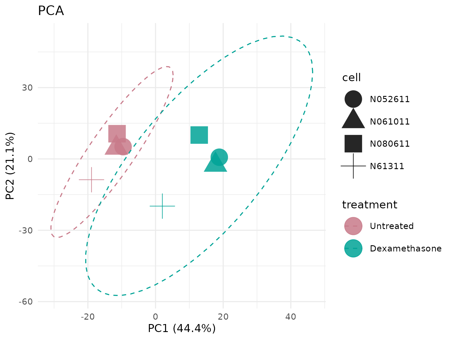
PCA with top variable genes
# Use top 500 most variable genes
get_pca_plot(
  vista,
  top_n_genes = 500,
  show_clusters = TRUE,
  shape_by = "cell"
)
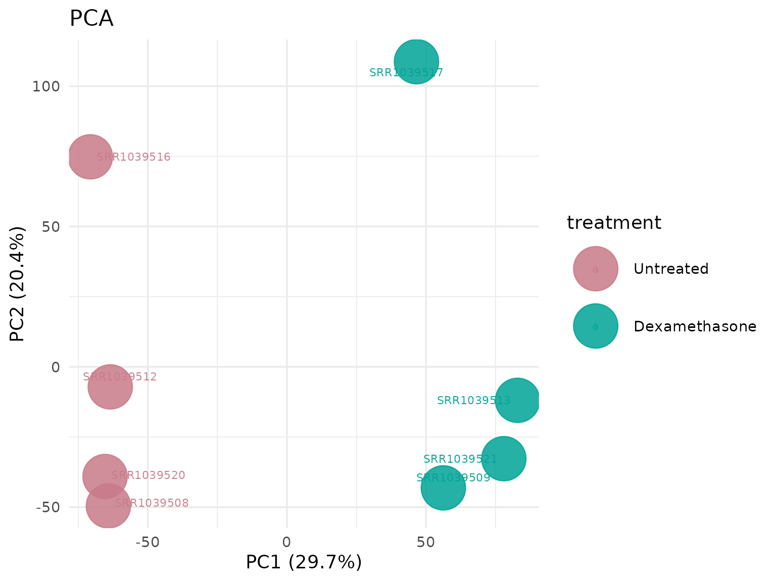
PCA with custom circle size
# Larger points for better visibility
get_pca_plot(
  vista,
  label = TRUE,
  point_size = 15,label_size = 5
)
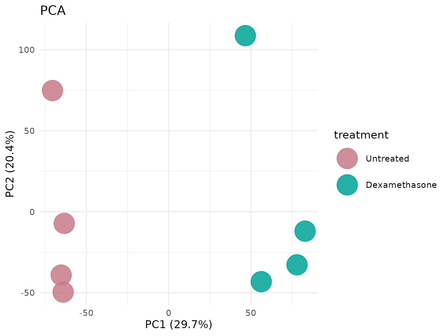
PCA without labels
# Clean plot without sample labels
get_pca_plot(
  vista,
  label = FALSE,
  point_size = 12
)
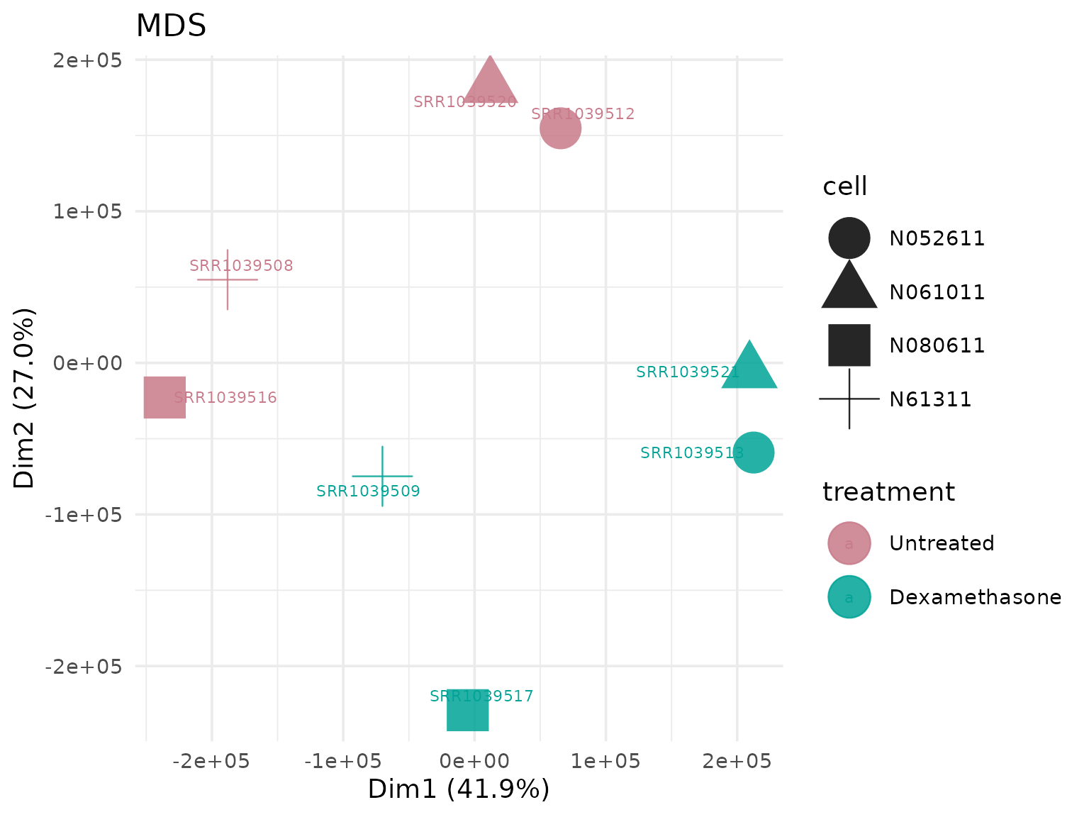
Multidimensional Scaling (MDS)
Alternative dimensionality reduction method.
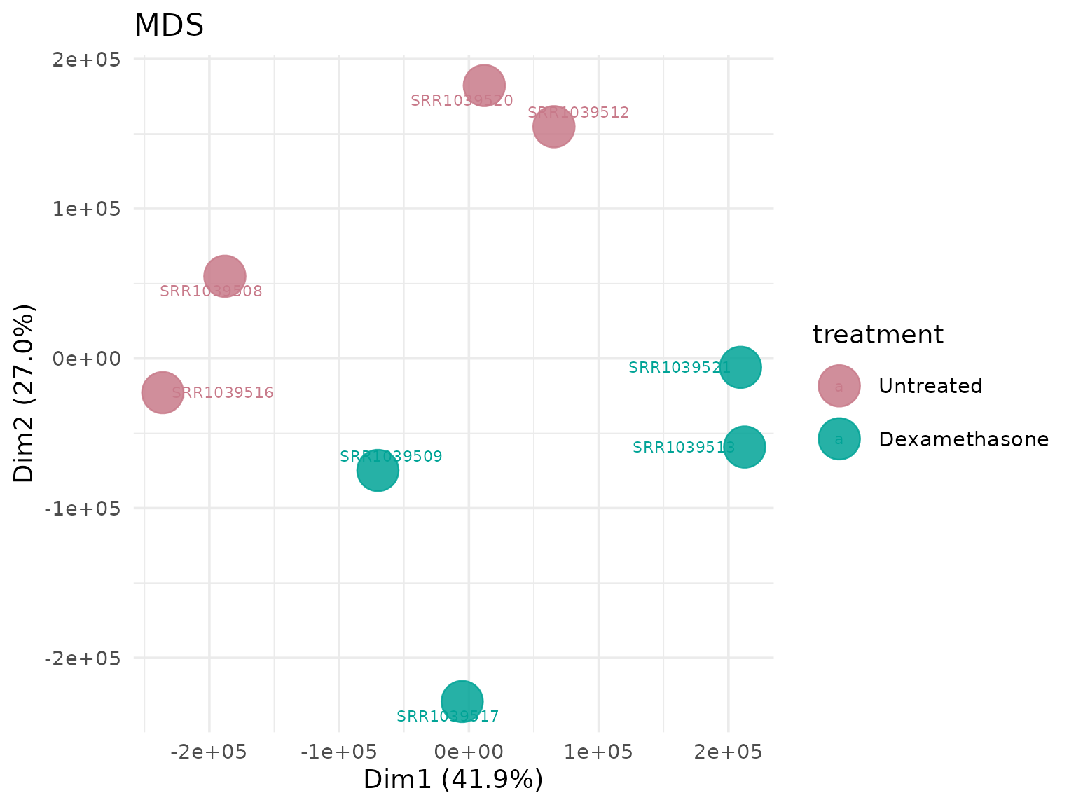
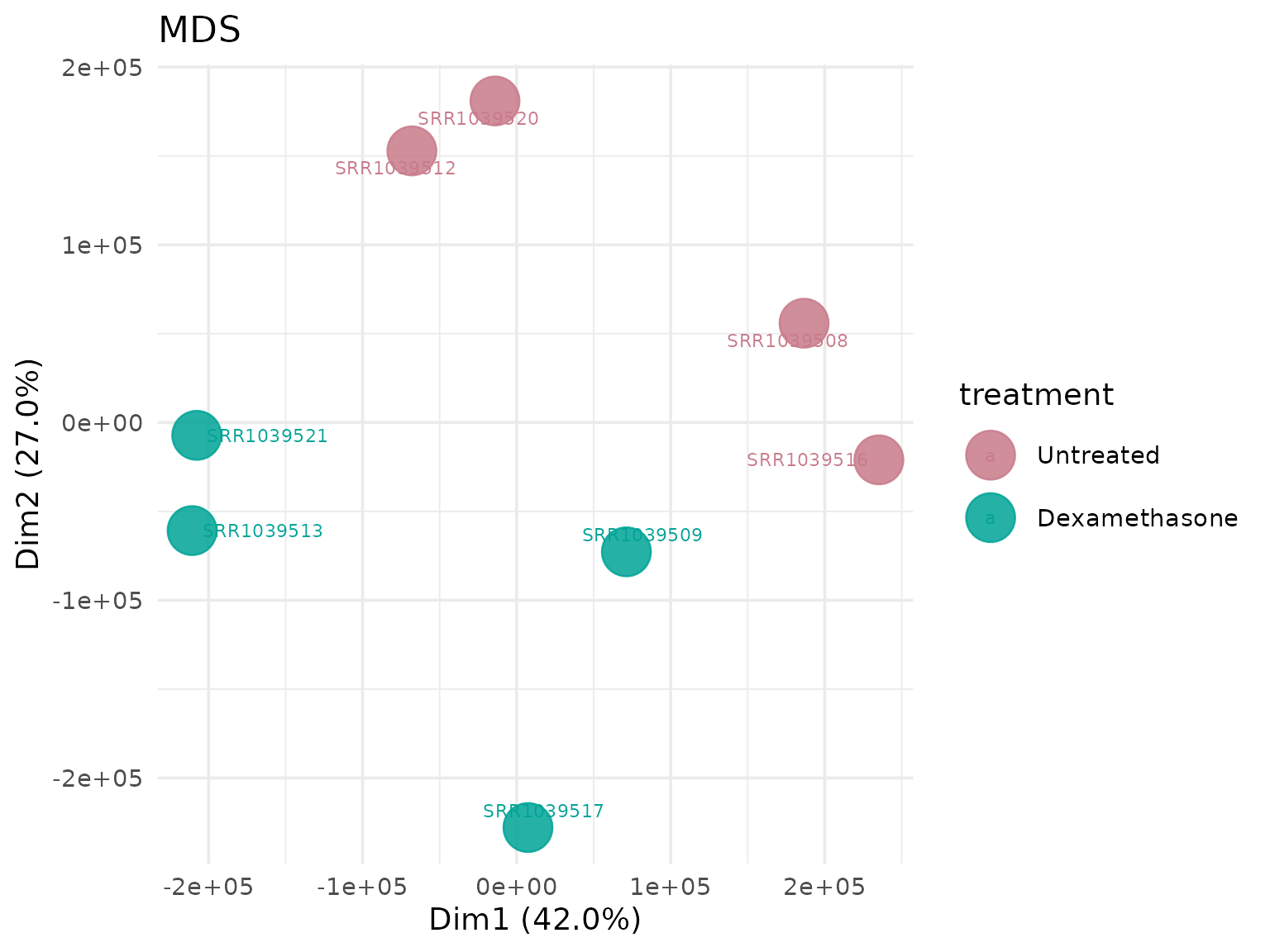
MDS with custom shapes
# Shape points by cell line
get_mds_plot(
  vista,
  label = TRUE,
  shape_by = "cell"
)
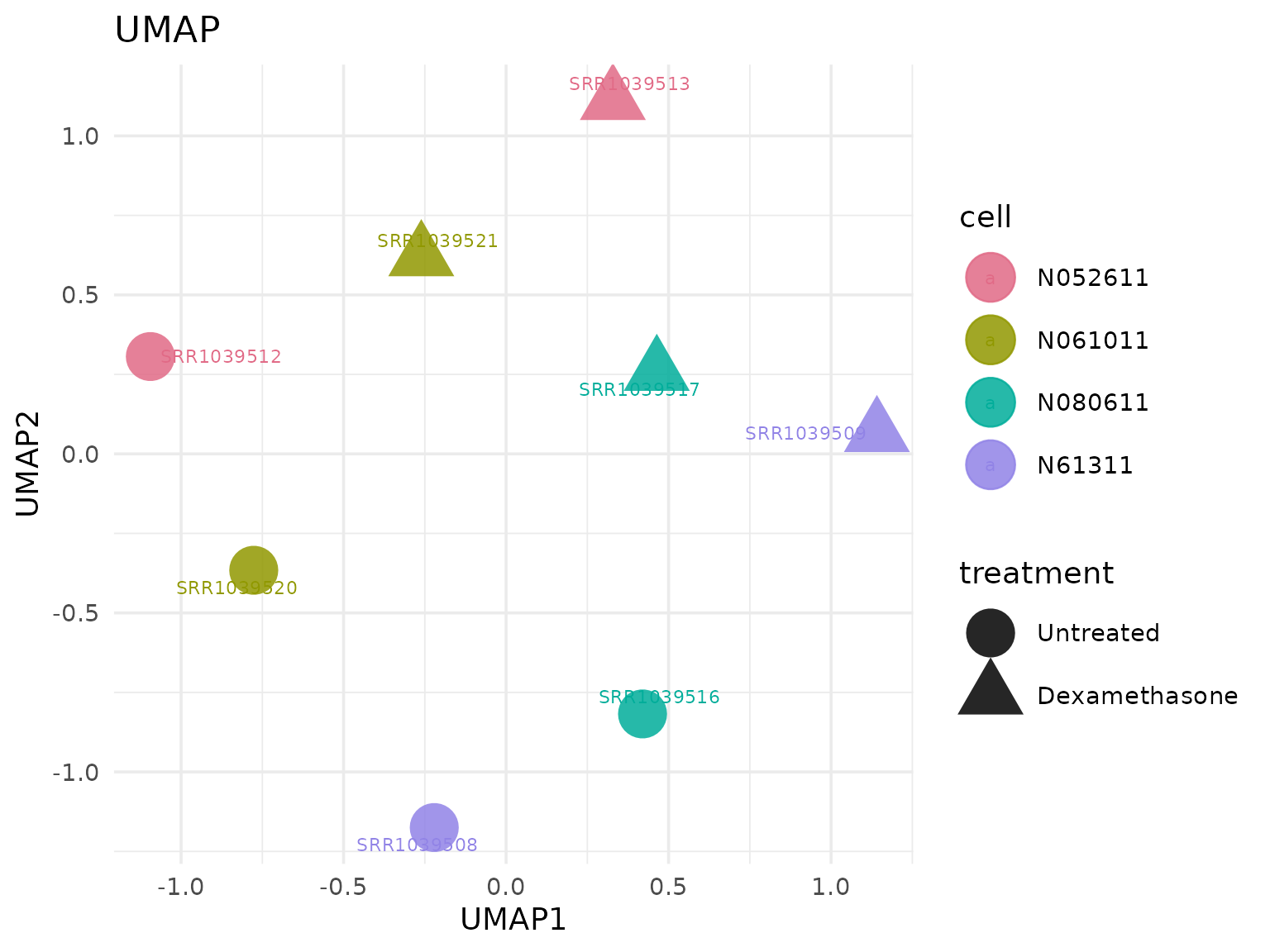
Uniform Manifold Approximation and Projection (UMAP)
Non-linear sample embedding for exploratory structure.
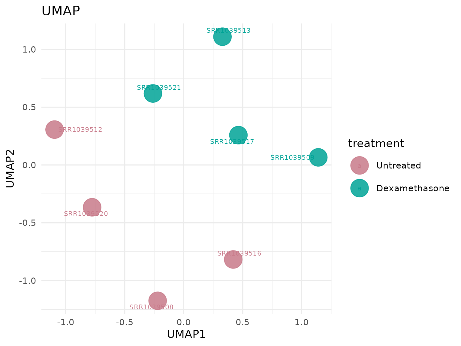
UMAP colored by a user-defined metadata column
get_umap_plot(
  vista,
  color_by = "cell",
  shape_by = "treatment",
  label = TRUE
)
Differential Expression Visualizations
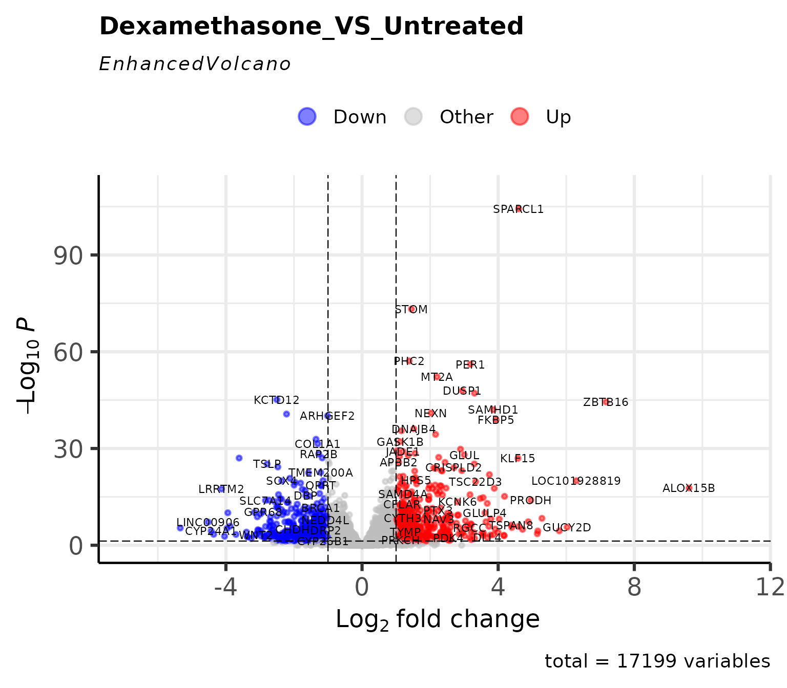
Volcano Plot
Classic volcano plot showing log2FC vs -log10(p-value).
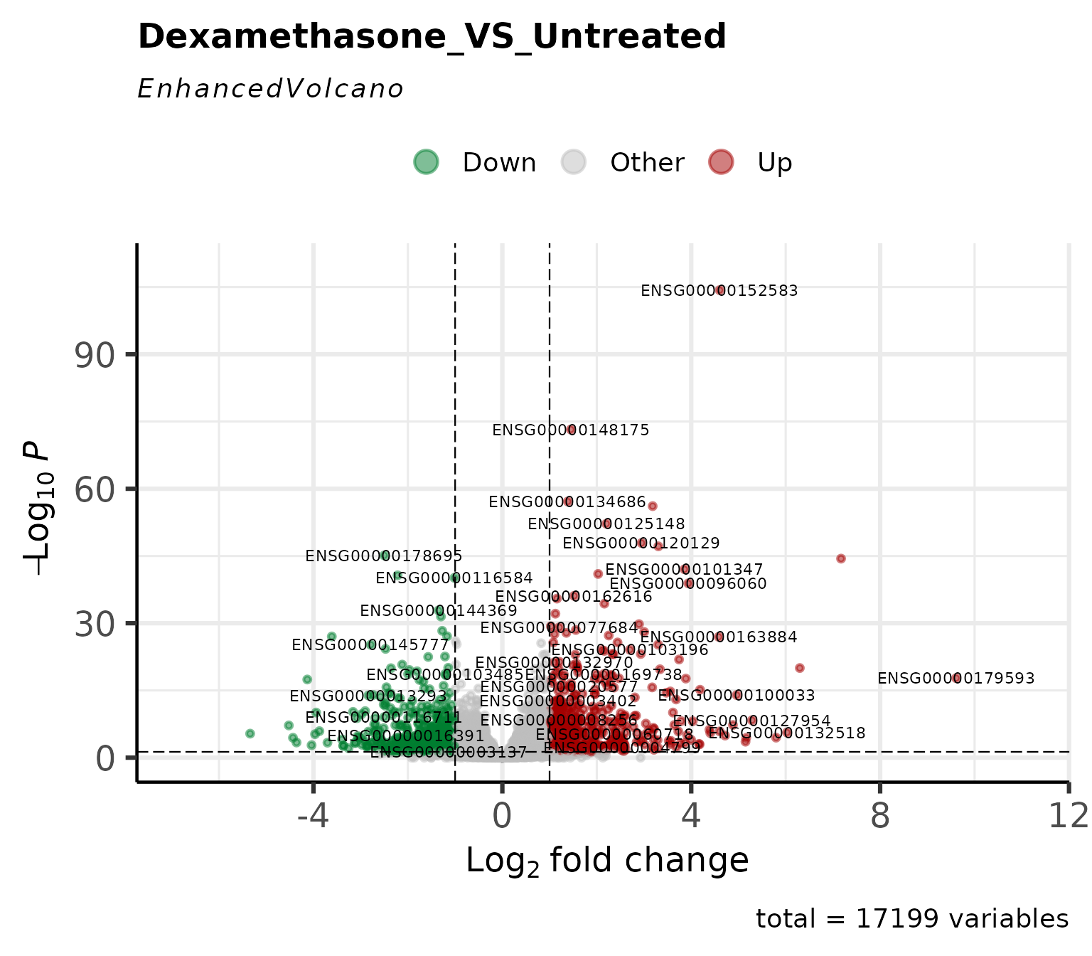
Customize cutoffs and labels
get_volcano_plot(
  vista,
  sample_comparison = comp_names[1],
  log2fc_cutoff = 1.5,
  pval_cutoff = 0.01,
  label_size = 3,
  display_id = "SYMBOL"
)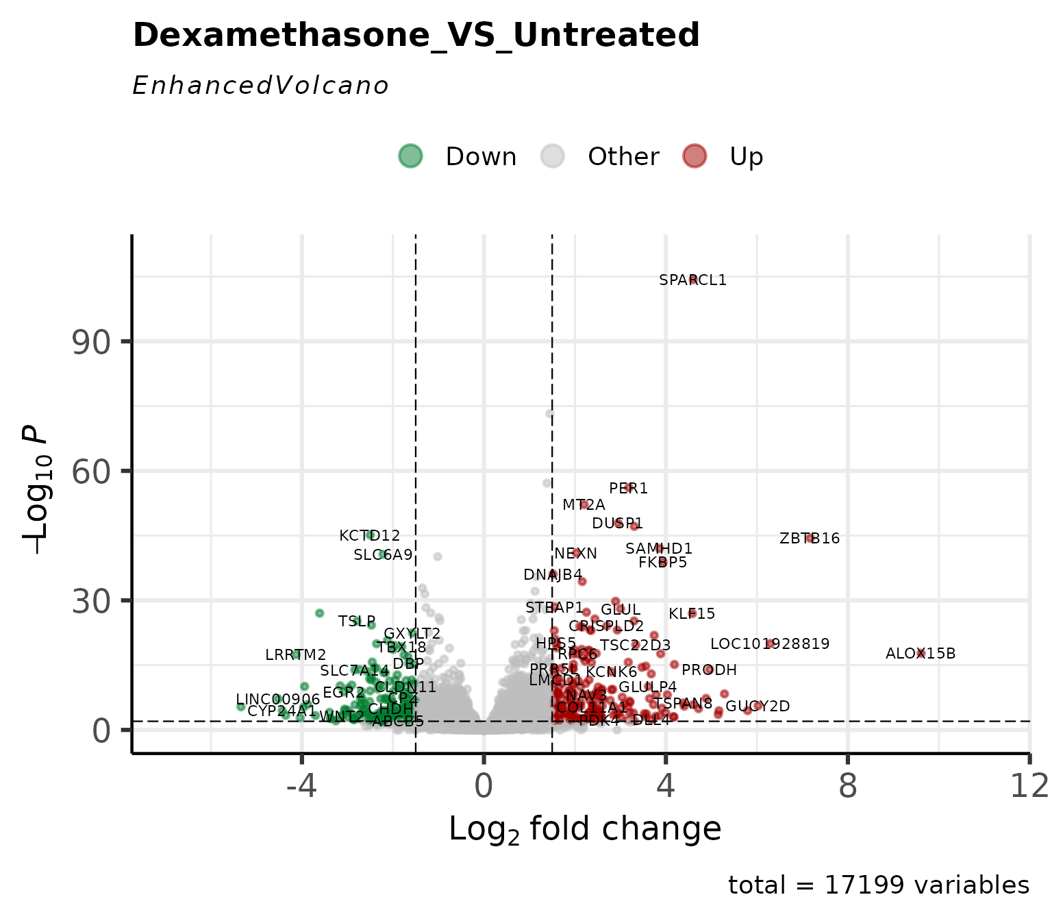
Custom colors
# Custom colors for up/down regulated genes
get_volcano_plot(
  vista,
  sample_comparison = comp_names[1],
  col_up = "red",
  col_down = "blue",
  display_id = "SYMBOL"
)
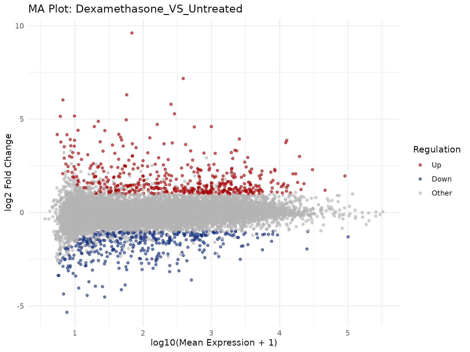
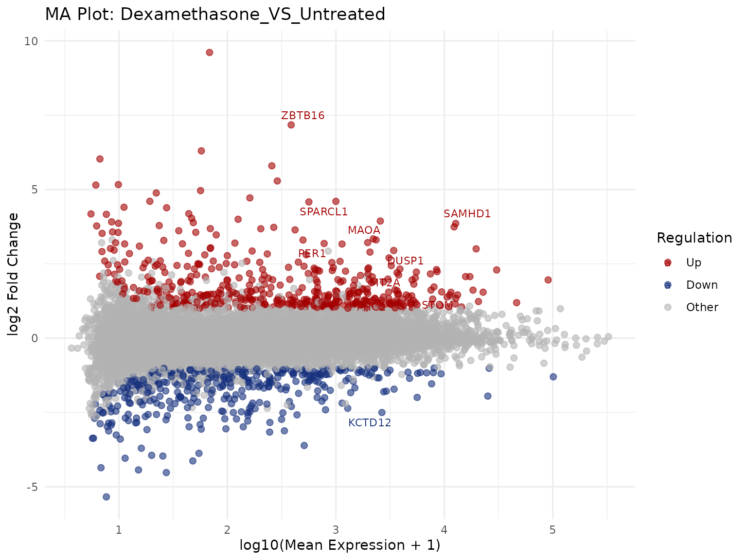
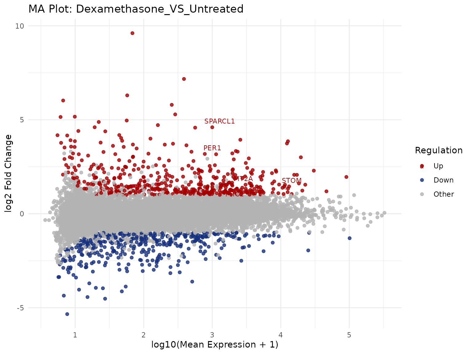
MA Plot
Mean expression vs log2 fold-change.
Label top genes
get_ma_plot(
  vista,
  sample_comparison = comp_names[1],
  label_n = 10,
  point_size = 2,
  display_id = "SYMBOL"
)
Custom cutoffs
get_ma_plot(
  vista,
  sample_comparison = comp_names[1],
  label_n = 5,
  display_id = "SYMBOL",
  point_size = 1.5,
  alpha = 0.8
)
Expression Pattern Analysis
Prepare gene sets
# Get top 50 DEGs by adjusted p-value
de_table <- comparisons(vista)[[1]]

top_degs <- get_genes_by_regulation(vista, names(comparisons(vista))[1],regulation = "Both",top_n = 50)[[1]]  # top 50 by abs fold change

top_up <- get_genes_by_regulation(vista, names(comparisons(vista))[1],regulation = "Up",top_n = 50)[[1]]

top_down <- get_genes_by_regulation(vista, names(comparisons(vista))[1],regulation = "Down",top_n = 50)[[1]]


cat("Top upregulated genes:\n")
#> Top upregulated genes:
print(top_up)
#>  [1] "ENSG00000179593" "ENSG00000109906" "ENSG00000250978" "ENSG00000132518"
#>  [5] "ENSG00000171819" "ENSG00000127954" "ENSG00000249364" "ENSG00000137673"
#>  [9] "ENSG00000100033" "ENSG00000168481" "ENSG00000168309" "ENSG00000264868"
#> [13] "ENSG00000152583" "ENSG00000163884" "ENSG00000177575" "ENSG00000127324"
#> [17] "ENSG00000101342" "ENSG00000270689" "ENSG00000268894" "ENSG00000152779"
#> [21] "ENSG00000128045" "ENSG00000096060" "ENSG00000152463" "ENSG00000173838"
#> [25] "ENSG00000273259" "ENSG00000101347" "ENSG00000187288" "ENSG00000219565"
#> [29] "ENSG00000211445" "ENSG00000143127" "ENSG00000128917" "ENSG00000170214"
#> [33] "ENSG00000163083" "ENSG00000178723" "ENSG00000248187" "ENSG00000157152"
#> [37] "ENSG00000170323" "ENSG00000231246" "ENSG00000233117" "ENSG00000157514"
#> [41] "ENSG00000189221" "ENSG00000165995" "ENSG00000182836" "ENSG00000112936"
#> [45] "ENSG00000269289" "ENSG00000174697" "ENSG00000179094" "ENSG00000187193"
#> [49] "ENSG00000006788" "ENSG00000102760"
cat("\nTop downregulated genes:\n")
#>
#> Top downregulated genes:
print(top_down)
#>  [1] "ENSG00000128285" "ENSG00000267339" "ENSG00000019186" "ENSG00000183454"
#>  [5] "ENSG00000146006" "ENSG00000122679" "ENSG00000155897" "ENSG00000143494"
#>  [9] "ENSG00000141469" "ENSG00000108700" "ENSG00000162692" "ENSG00000175489"
#> [13] "ENSG00000183092" "ENSG00000250657" "ENSG00000136267" "ENSG00000214814"
#> [17] "ENSG00000261121" "ENSG00000105989" "ENSG00000122877" "ENSG00000188176"
#> [21] "ENSG00000131771" "ENSG00000165272" "ENSG00000184564" "ENSG00000079101"
#> [25] "ENSG00000188501" "ENSG00000119714" "ENSG00000223811" "ENSG00000130487"
#> [29] "ENSG00000166670" "ENSG00000165388" "ENSG00000013293" "ENSG00000123405"
#> [33] "ENSG00000145777" "ENSG00000140600" "ENSG00000124134" "ENSG00000146250"
#> [37] "ENSG00000116991" "ENSG00000126878" "ENSG00000197046" "ENSG00000128165"
#> [41] "ENSG00000084710" "ENSG00000173110" "ENSG00000123689" "ENSG00000106003"
#> [45] "ENSG00000181634" "ENSG00000154864" "ENSG00000182732" "ENSG00000136999"
#> [49] "ENSG00000015520" "ENSG00000095585"
Expression Heatmaps
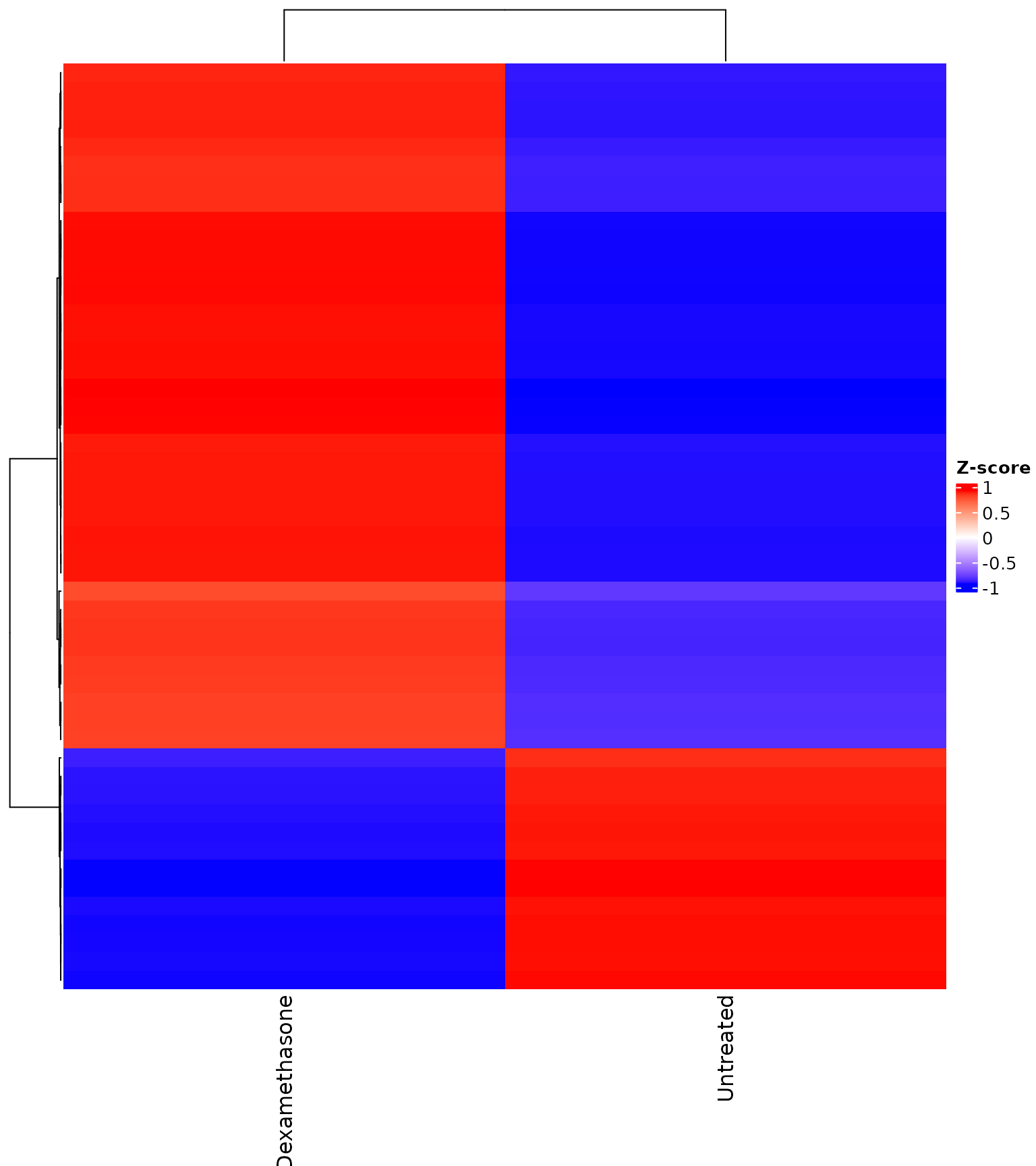
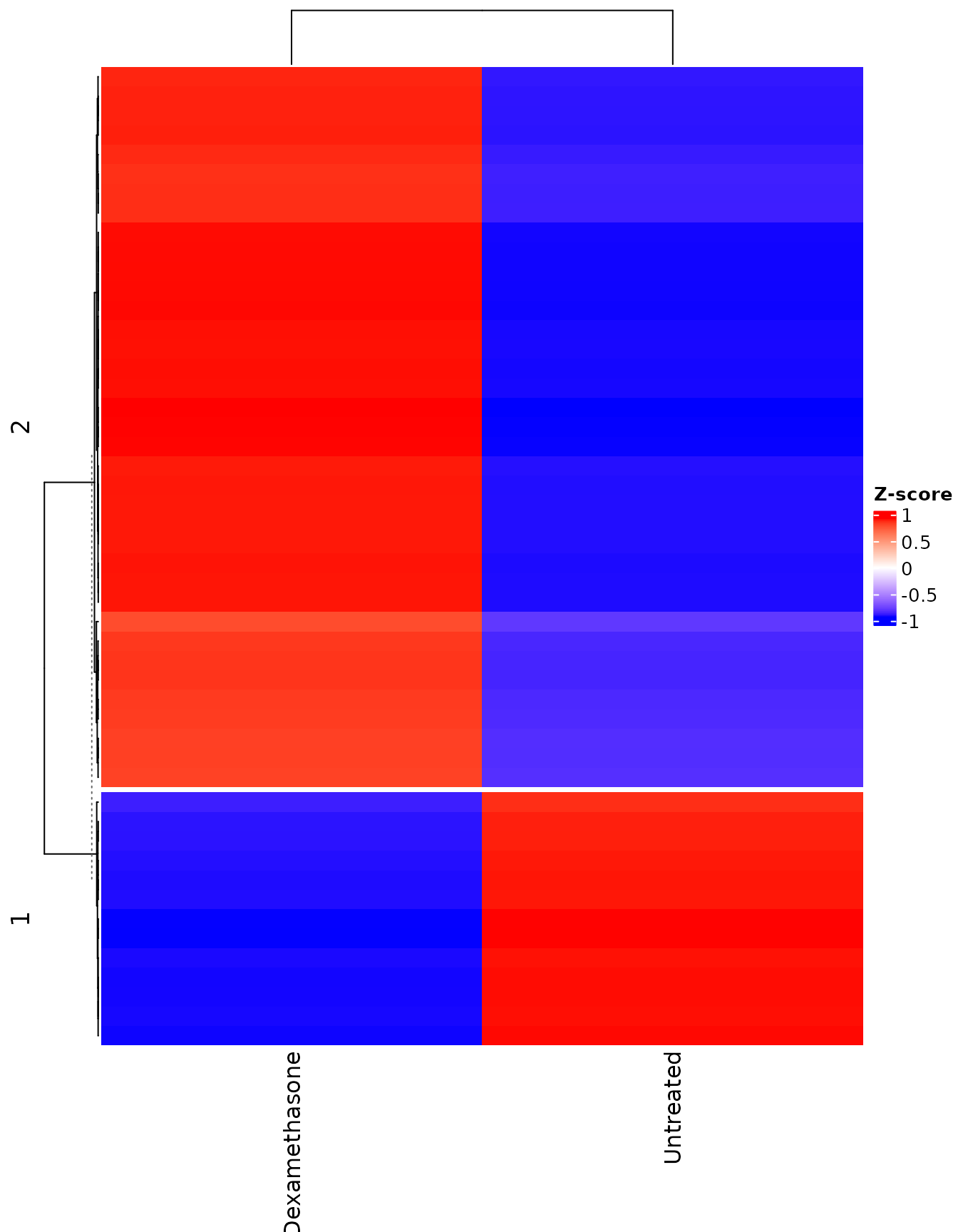
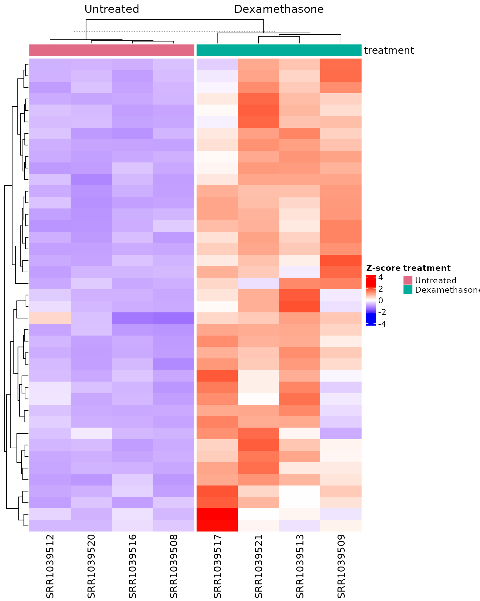
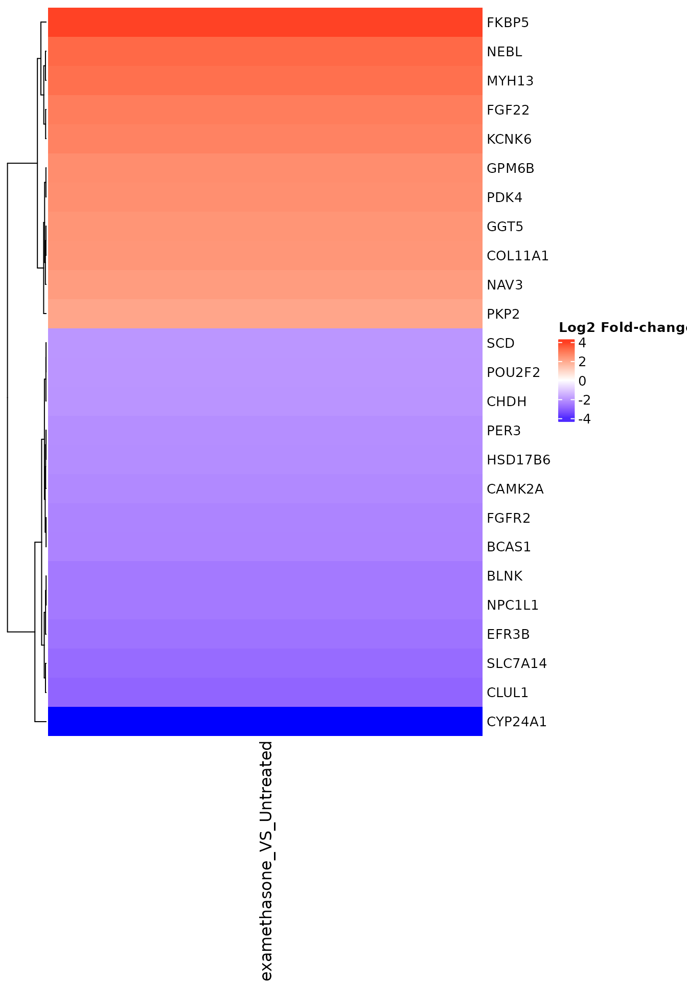
Heatmap with explicit gene set
get_expression_heatmap(
  vista,
  sample_group = levels(colData(vista)$treatment),
  genes = top_degs,
  display_id = "SYMBOL",
  show_row_names = TRUE
)
Heatmap with k-means clustering
get_expression_heatmap(
  vista,
  sample_group = levels(colData(vista)$treatment),
  genes = top_degs,
  display_id = "SYMBOL",
  kmeans_k = 3,
  show_row_names = TRUE
)
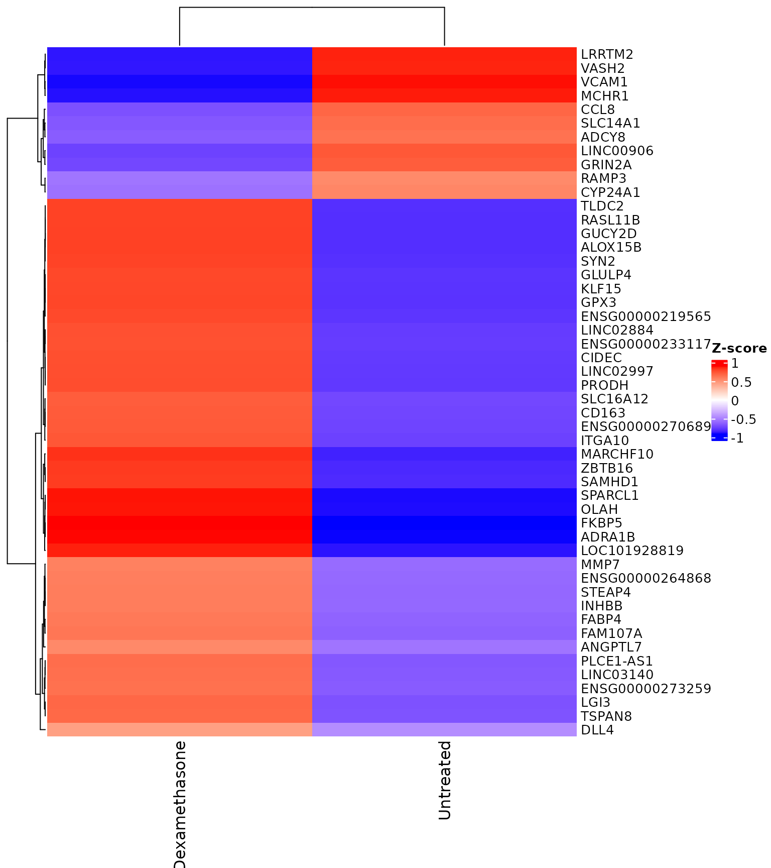
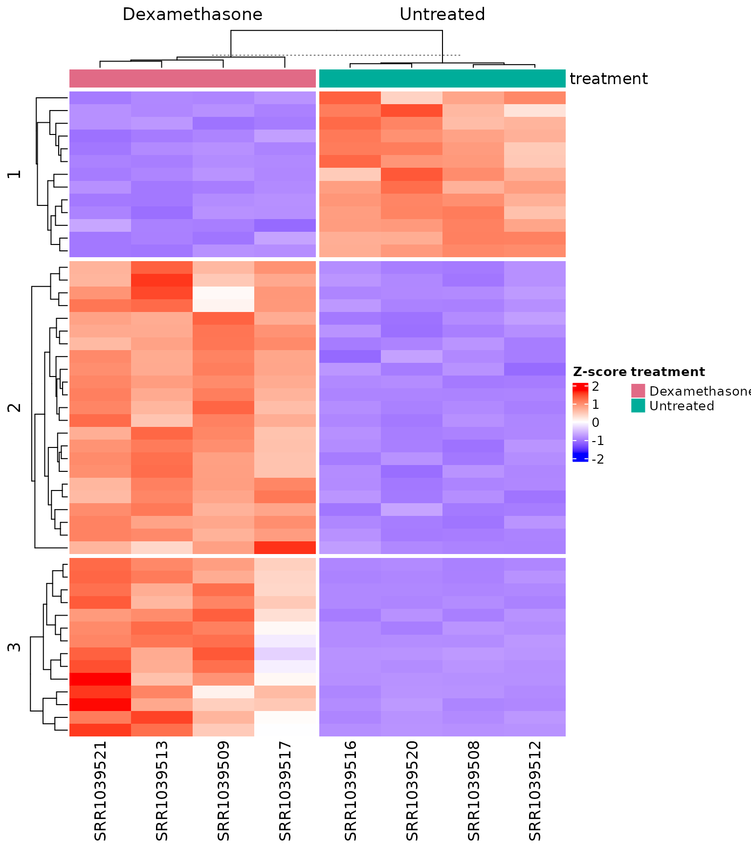
Heatmap with column annotations
get_expression_heatmap(
  vista,
  sample_group = levels(colData(vista)$treatment),
  genes = top_degs,
  show_row_names = TRUE,
  display_id = "SYMBOL",
  kmeans_k = 3,
  cluster_row_slice = FALSE,
  summarise_replicates = FALSE,
  annotate_columns = TRUE
)
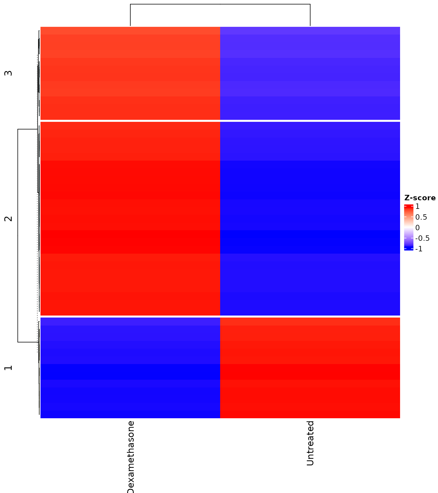
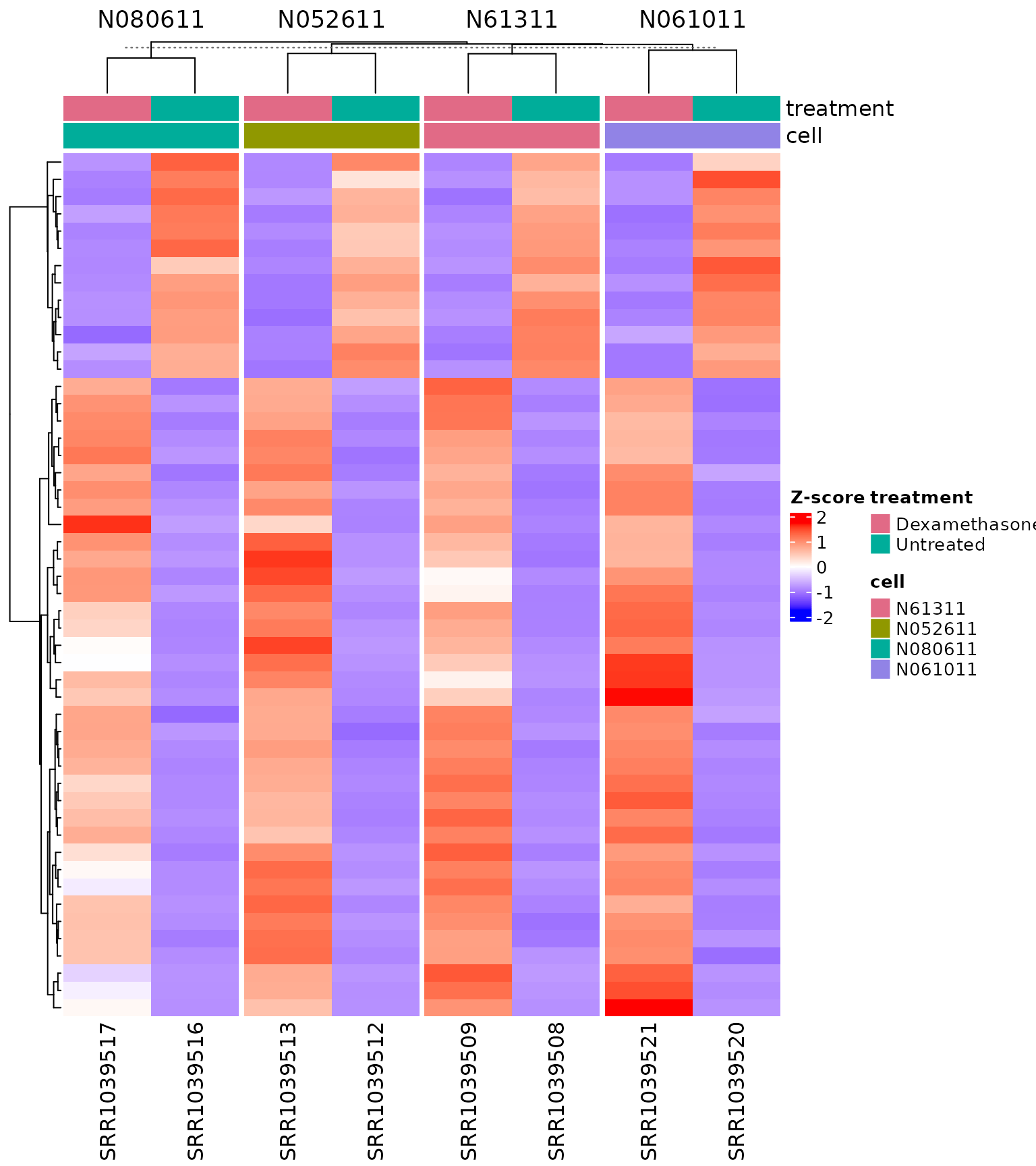
Heatmap with multiple column annotations and
cluster_by
# Use multiple sample-level columns in top annotation.
# By default, columns are split by the first annotation column.


get_expression_heatmap(
  vista,
  sample_group = levels(colData(vista)$treatment),
  genes = top_degs,
  show_row_names = FALSE,
  display_id = "SYMBOL",
  summarise_replicates = FALSE,
  annotate_columns = c("treatment", "cell"),
  cluster_by = "cell"
)
Heatmap showing each replicate
get_expression_heatmap(
  vista,
  sample_group = levels(colData(vista)$treatment),
  genes = top_degs,
  display_id = "SYMBOL",
  summarise_replicates = FALSE,
  show_row_names = FALSE,
  annotate_columns = TRUE,
  kmeans_k = 2
)
Expression Barplots
Basic barplot
get_expression_barplot(
  vista,
  genes = top_up[1:4],
  display_id = "SYMBOL",
)+theme_minimal(base_size = 16)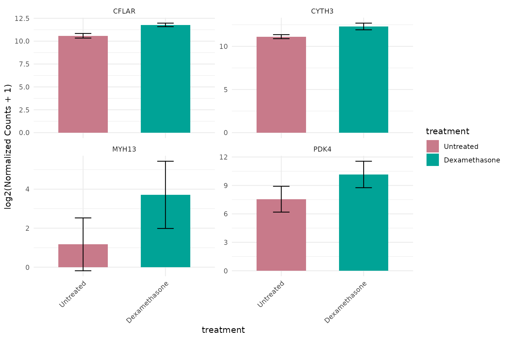
Log-transformed with statistics
# Add statistical comparisons between groups
get_expression_barplot(
  vista,
  genes = top_up[1:4],
  display_id = "SYMBOL",
  log_transform = TRUE,
  stats_group = TRUE  # Enable statistical annotations
) + theme_minimal(base_size = 16)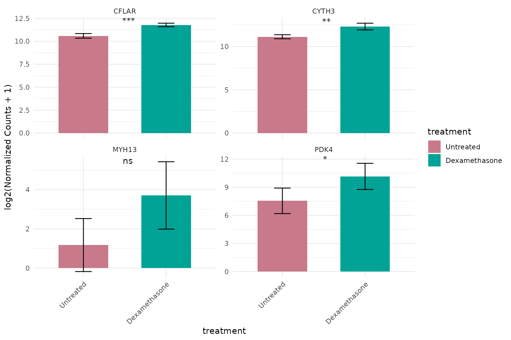
Per-sample barplot for selected genes
get_expression_barplot(
  vista,
  genes = top_up[1:2],
  display_id = "SYMBOL",
  by = "sample",
  sample_order = "group"
)+ theme(text = element_text(size = 16))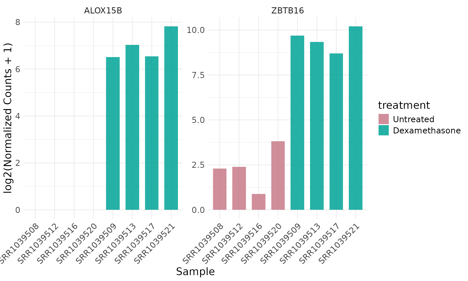
Compare up and down regulated genes
# Compare expression of both up- and down-regulated genes
selected_genes <- c(top_up[1:3], top_down[1:3])
get_expression_barplot(
  vista,
  genes = selected_genes,
  display_id = "SYMBOL",
  log_transform = TRUE,
  stats_group = TRUE
)+ theme(text = element_text(size = 16))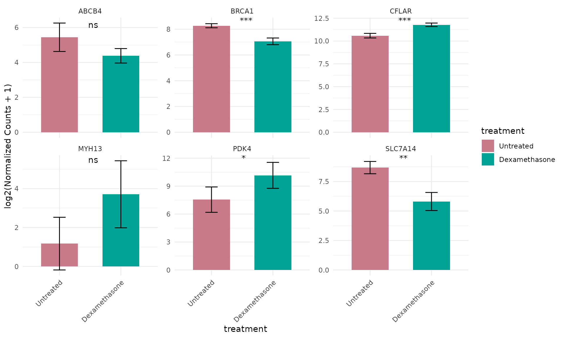
Expression Boxplots
Basic boxplot
get_expression_boxplot(
  vista,
  genes = top_up[1:4],
  display_id = "SYMBOL"
)+ theme(text = element_text(size = 16))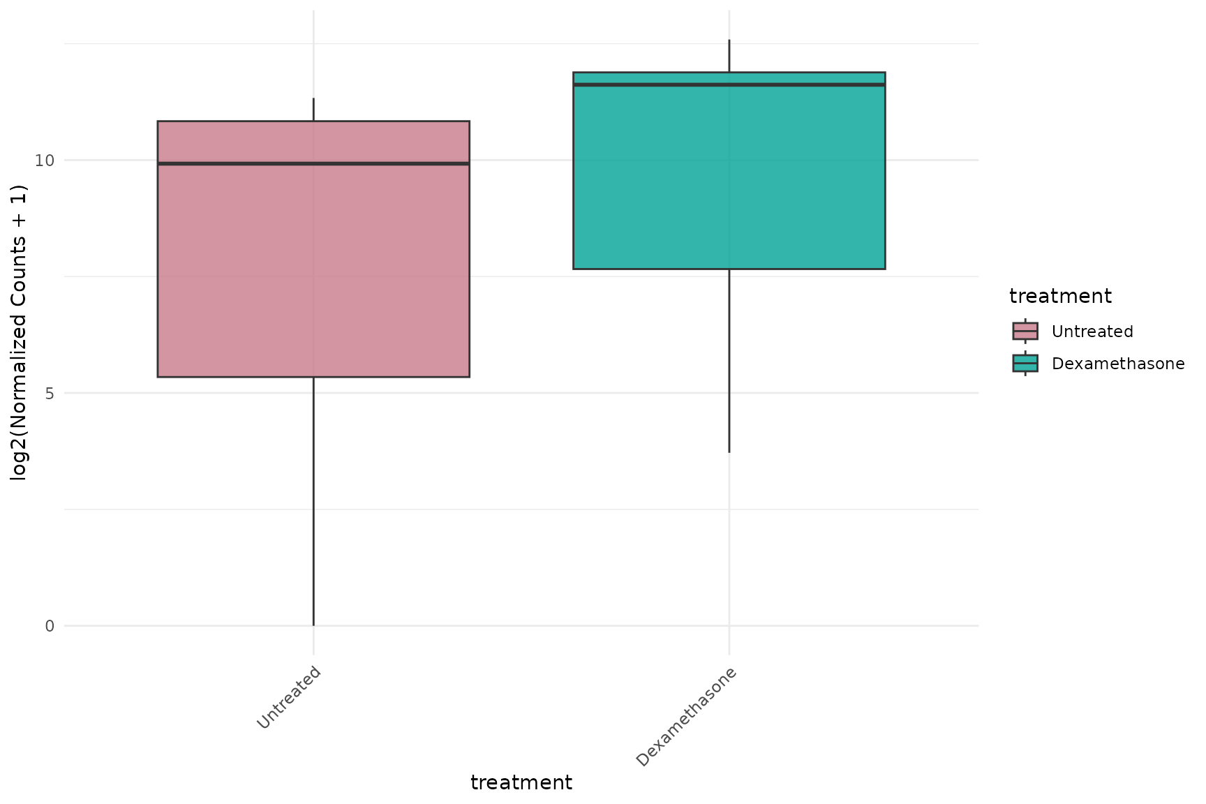
Boxplot without faceting
# All genes overlaid on same plot
get_expression_boxplot(
  vista,
  genes = top_up[1:3],
  display_id = "SYMBOL",
  facet_by = "none"
) + theme(text = element_text(size = 16))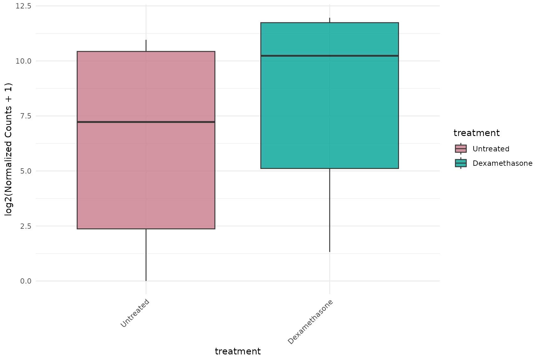
Boxplot with faceting by gene
# Each gene in separate panel - must specify facet_by = "gene"
get_expression_boxplot(
  vista,
  genes = top_up[1:3],
  display_id = "SYMBOL",
  facet_by = "gene",
  facet_scales = "free_y"
) + theme(text = element_text(size = 16))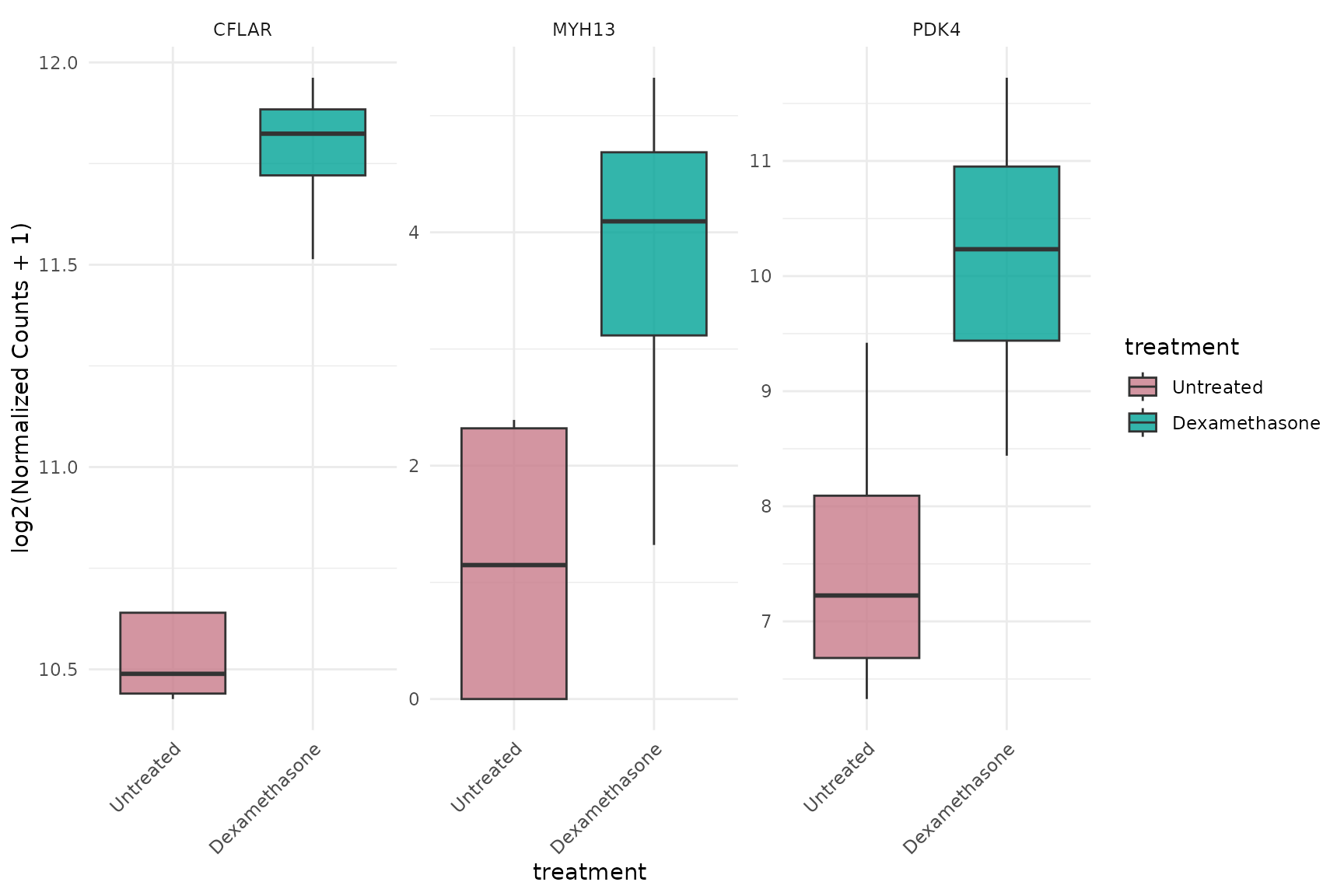
Boxplot with gene facets AND statistics
# Each gene in separate panel WITH statistical comparisons
get_expression_boxplot(
  vista,
  genes = top_up[1:4],
  display_id = "SYMBOL",
  log_transform = TRUE,
  facet_by = "gene",
  facet_scales = "free_y",
  stats_group = TRUE,  # Add statistics to each gene panel
  p.label = "p.signif"
)+ theme(text = element_text(size = 16))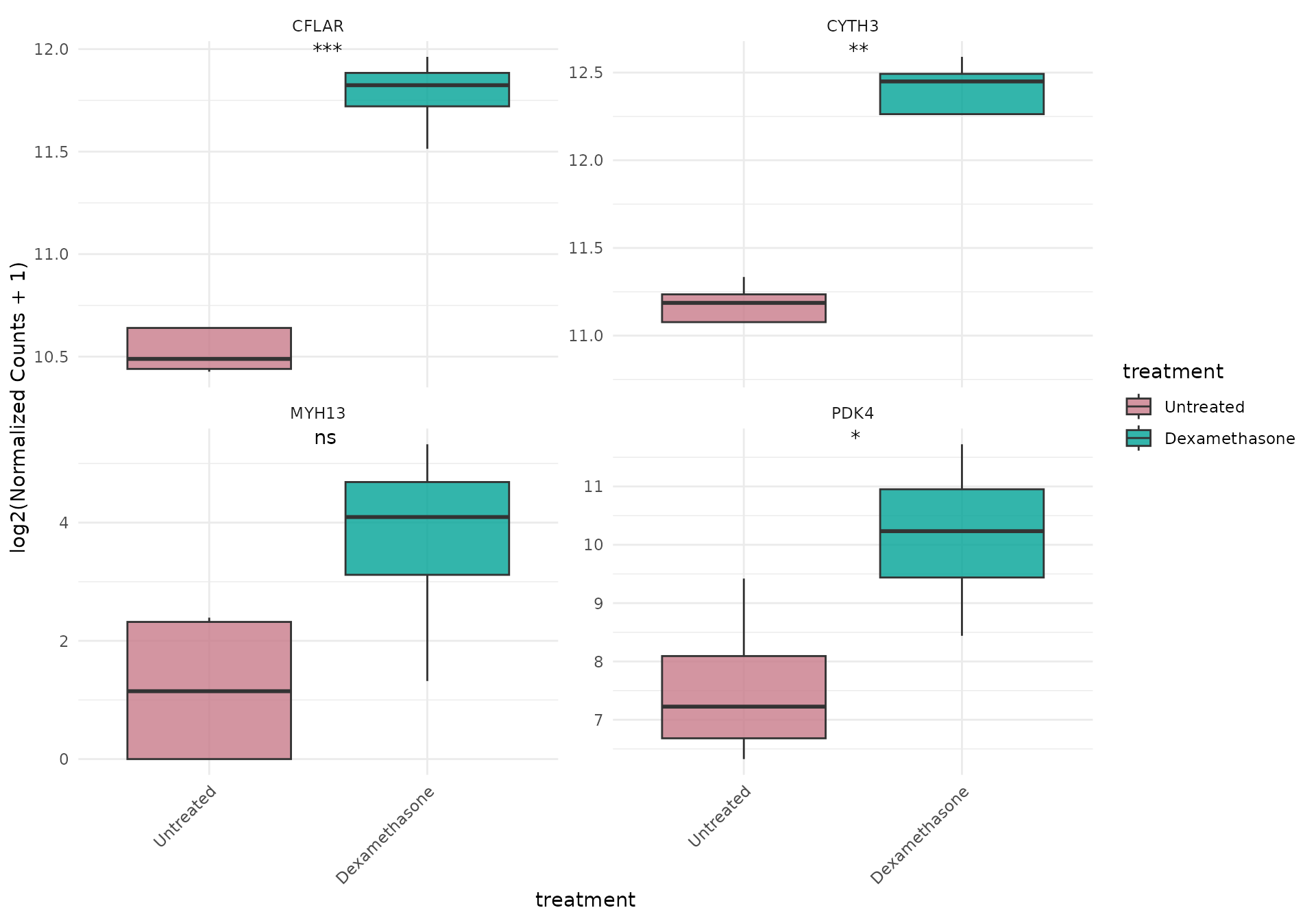
Pooled genes with statistics
# Pool all genes together for group comparison with statistical test
get_expression_boxplot(
  vista,
  genes = top_up[1:5],
  display_id = "SYMBOL",
  log_transform = TRUE,
  pool_genes = TRUE,
  facet_by = "none",
  stats_group = TRUE,  # Required for statistical annotations
  p.label = "p.signif"
)+ theme(text = element_text(size = 16))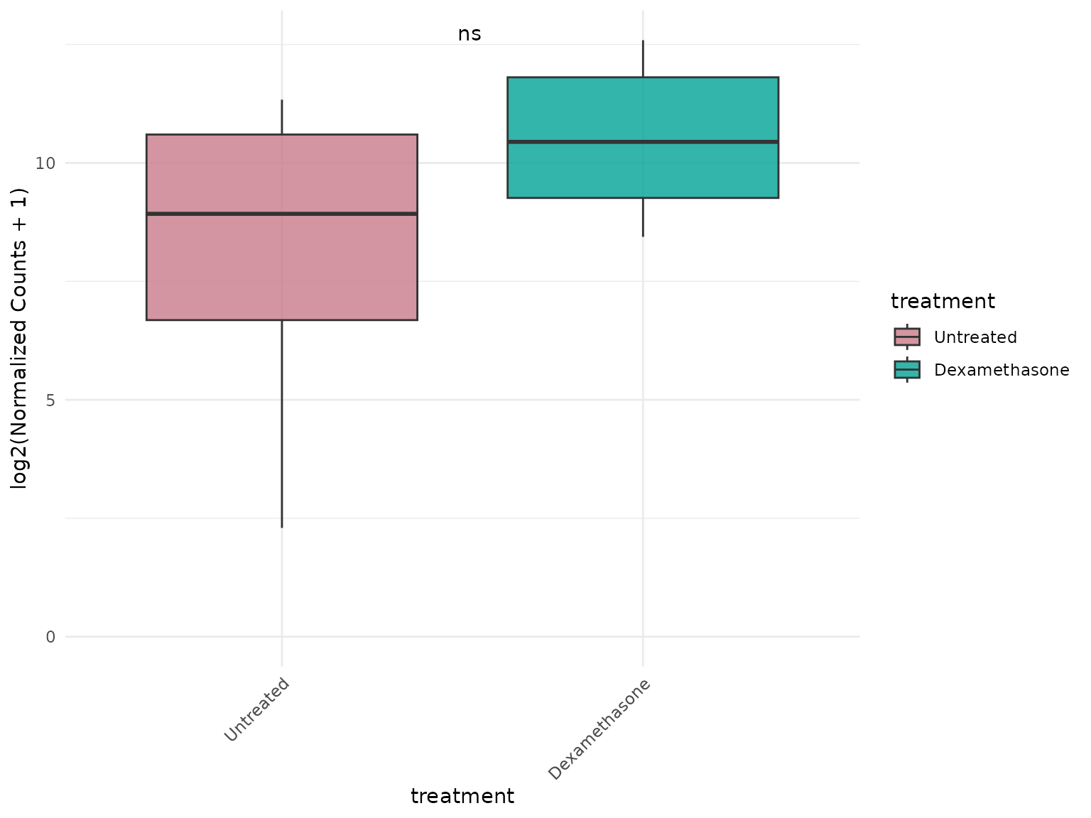
Log-transformed with p-values
# Show statistical comparisons between treatment groups
get_expression_boxplot(
  vista,
  genes = top_up[1:4],
  display_id = "SYMBOL",
  log_transform = TRUE,
  stats_group = TRUE,  # Enable statistical annotations
  p.label = "p.signif"
)+ theme(text = element_text(size = 16))
Expression Violin Plots
Basic violin plot
get_expression_violinplot(
  vista,
  genes = top_up[1:4],
  display_id = "SYMBOL"
)+ theme(text = element_text(size = 16))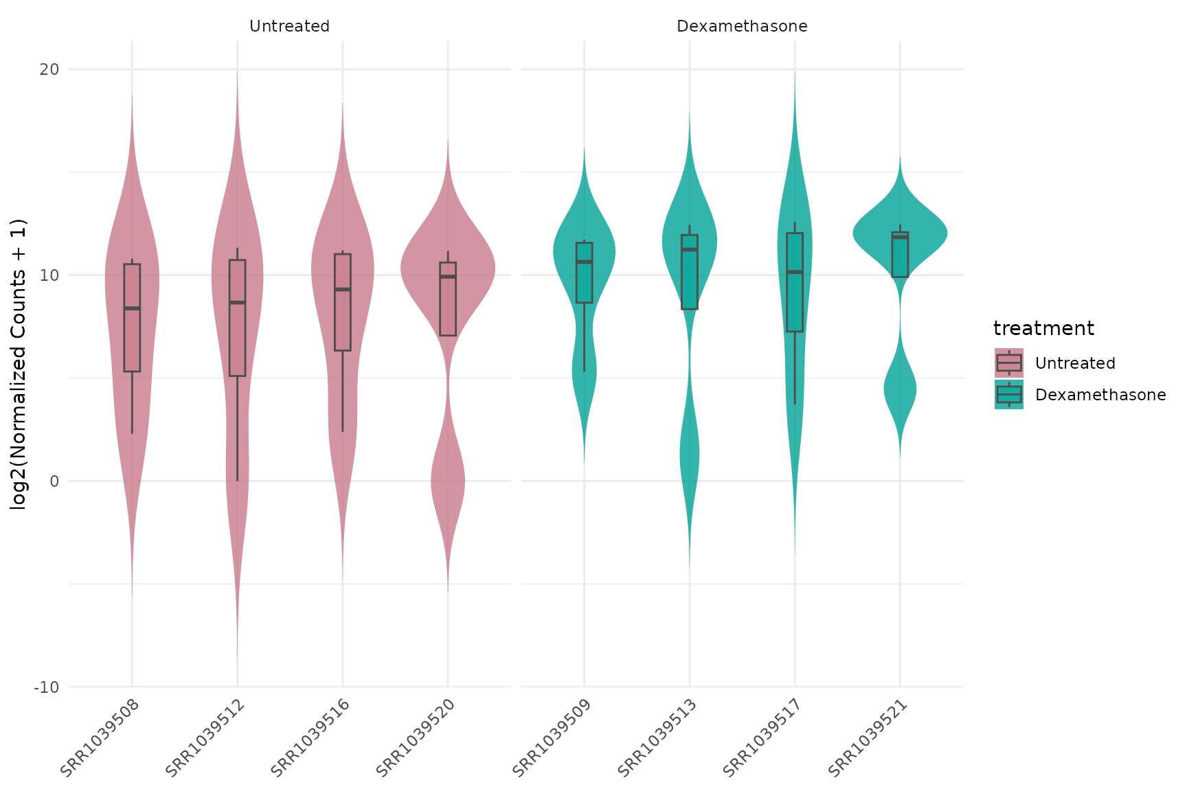
Violin with log2 transformation
get_expression_violinplot(
  vista,
  genes = top_up[1:4],,
  display_id = "SYMBOL",
  value_transform = "none"
)+ theme(text = element_text(size = 16))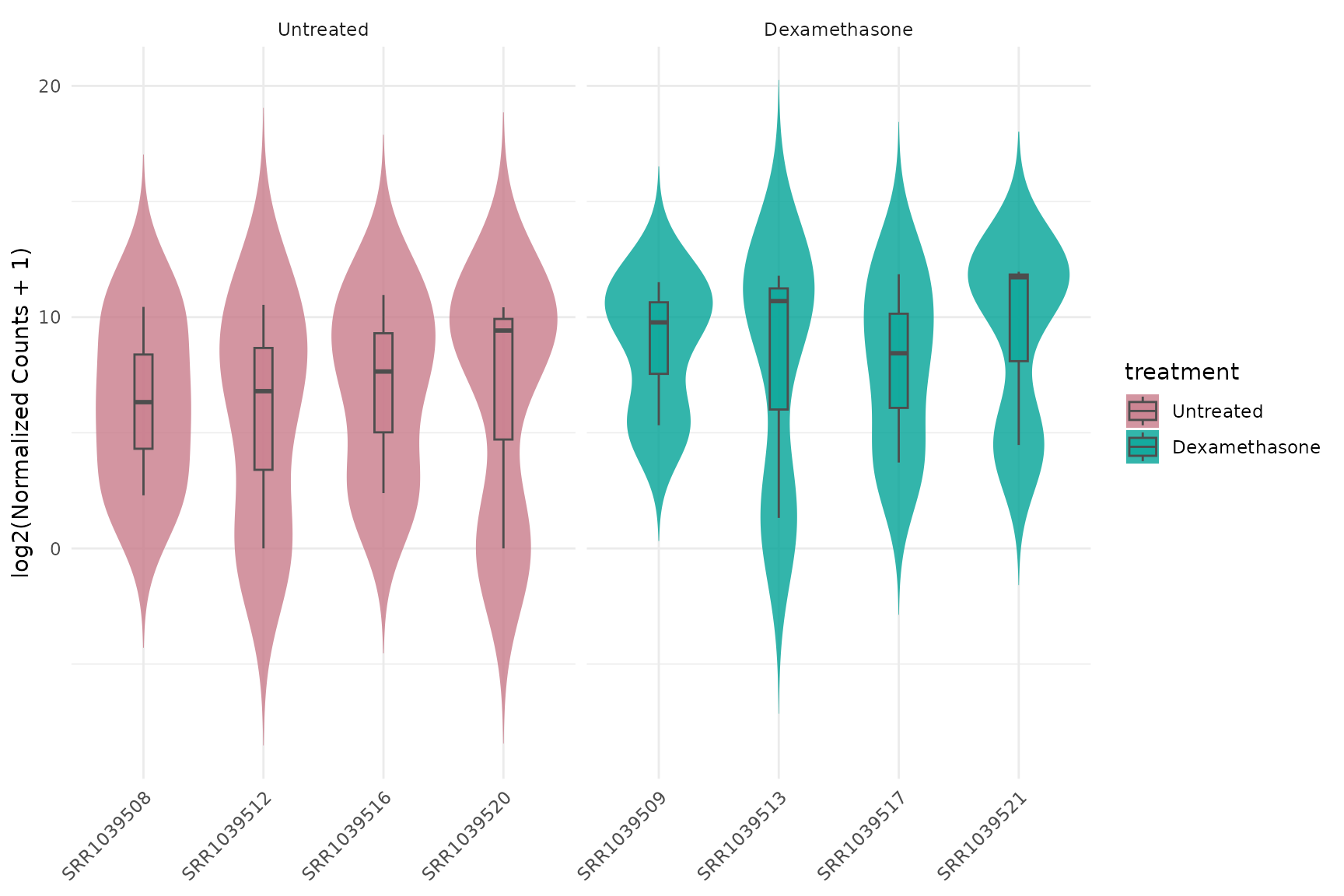
Violin with z-score transformation
get_expression_violinplot(
  vista,
  genes = top_up[1:4],
  value_transform = "zscore"
)+ theme(text = element_text(size = 16))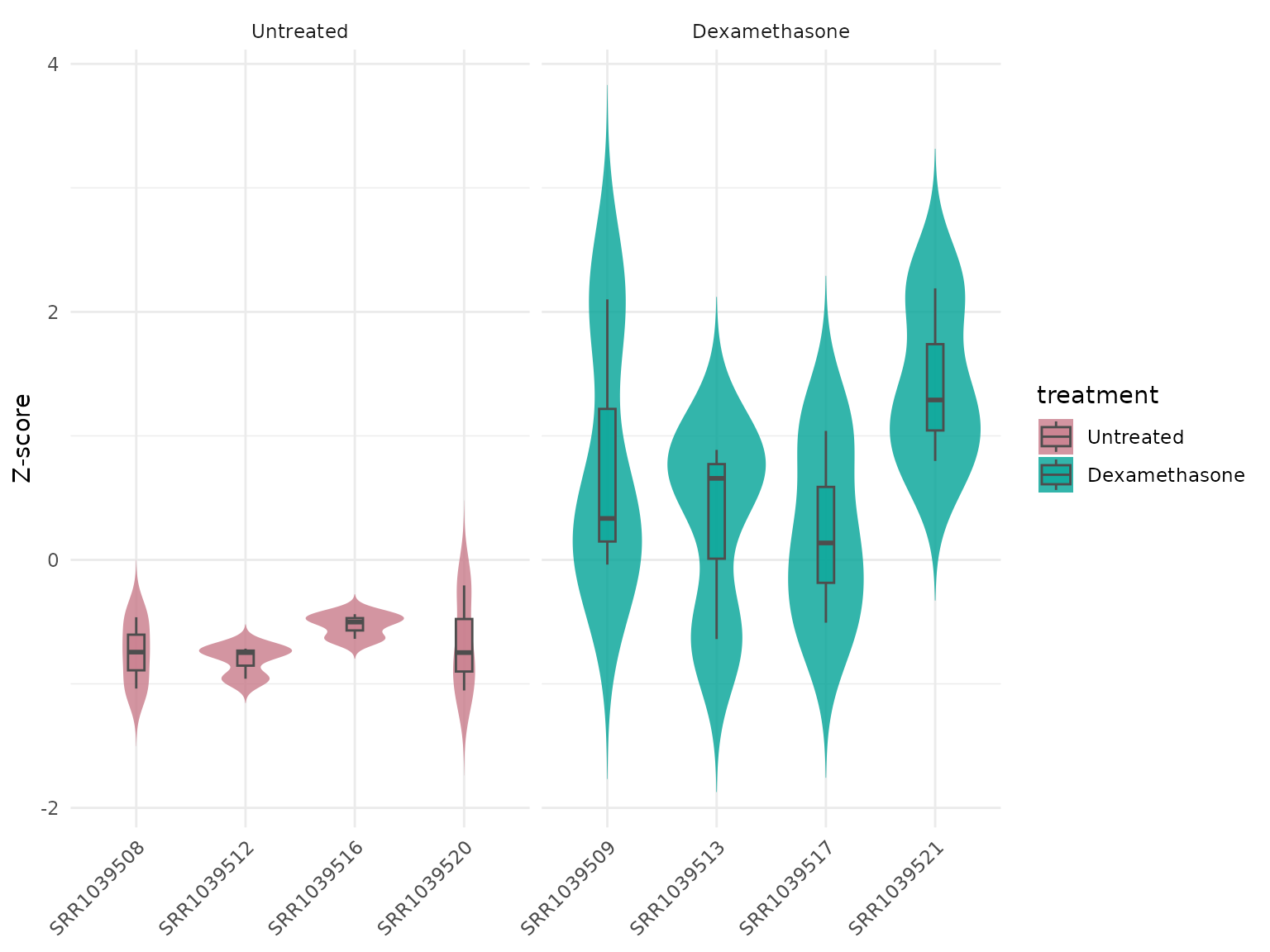
Additional Expression Plots
Density plot
get_expression_density(
  vista,
  genes = top_up[1:50],
  log_transform = TRUE
)+ theme(text = element_text(size = 16))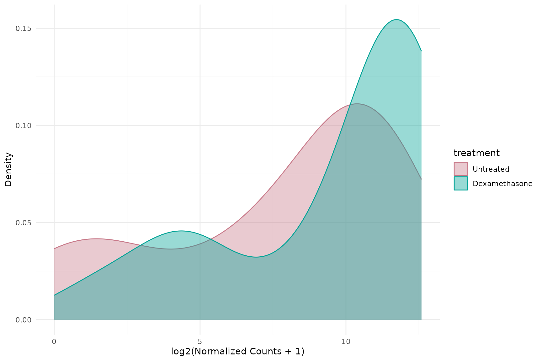
Scatter plot (sample vs sample)
# Compare two samples
samples <- colnames(vista)
get_expression_scatter(
  vista,
  sample_x = samples[1],
  sample_y = samples[2],
  log_transform = TRUE,
  label_n = 50,display_id = "SYMBOL",label_size = 4
)+ theme(text = element_text(size = 16))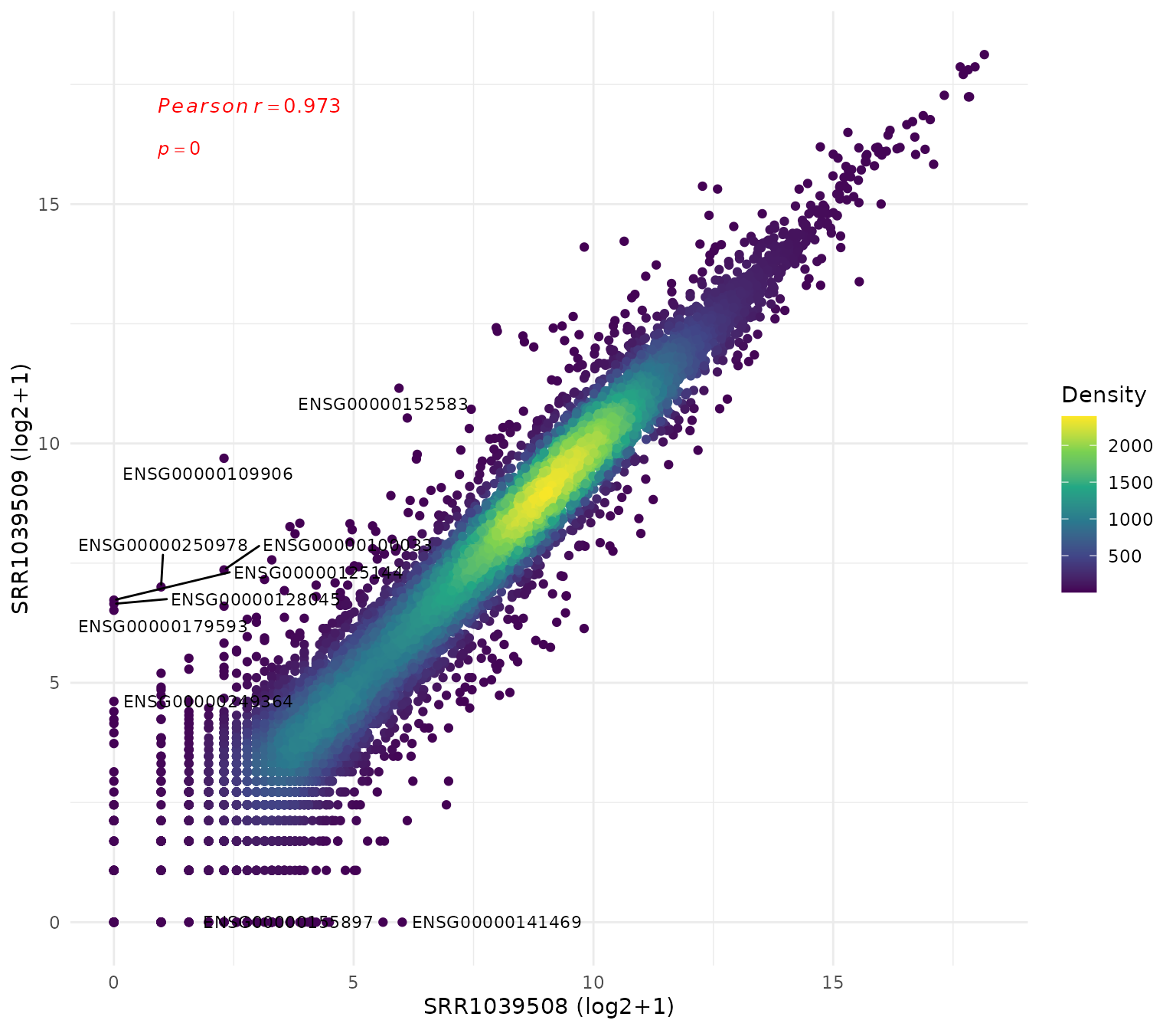
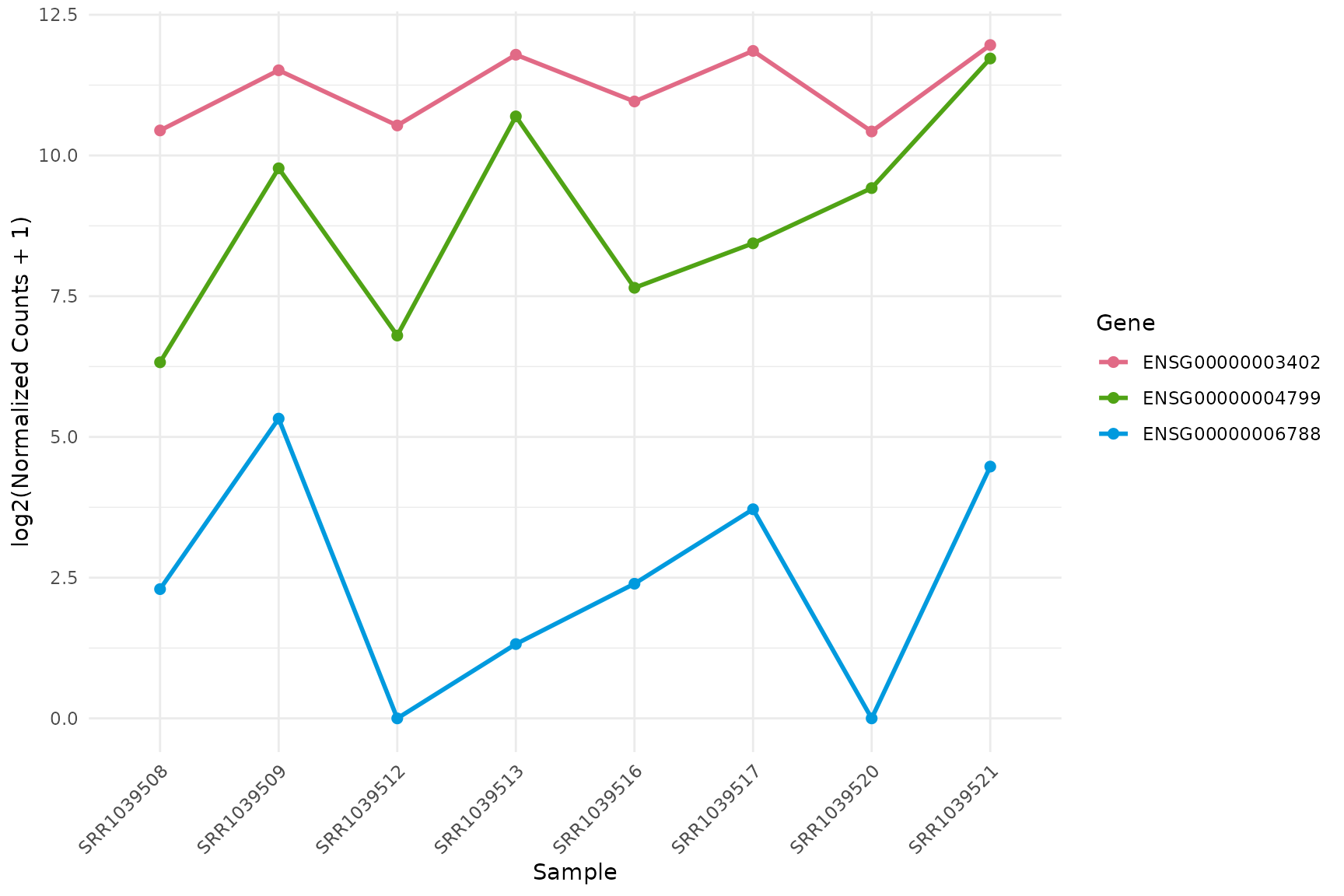
Line plot (expression across samples)
get_expression_lineplot(
  vista,
  genes = top_up[1:3],
  log_transform = TRUE,display_id = "SYMBOL",
  by = "sample",facet_by = "none",
  group_column = "treatment",sample_group = c("Untreated","Dexamethasone")
)
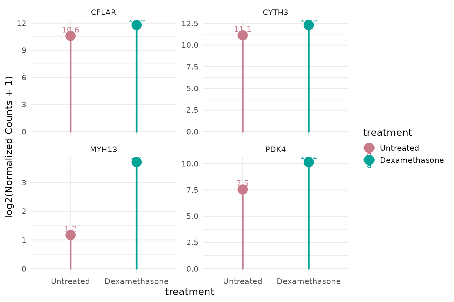
Lollipop plot
get_expression_lollipop(
  vista,
  genes = top_up[1:4],
  display_id = "SYMBOL",
  log_transform = TRUE
)
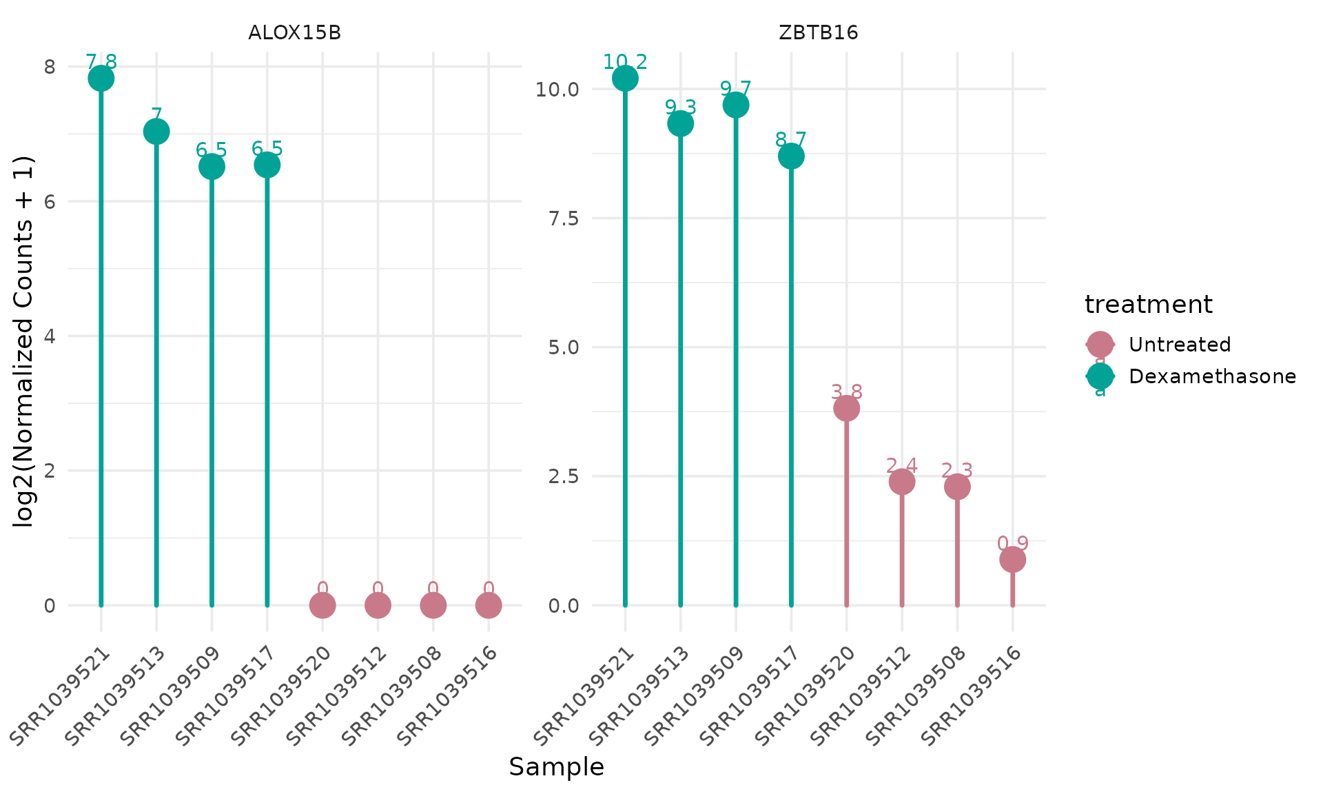
Per-sample lollipop plot
get_expression_lollipop(
  vista,
  genes = top_up[1:2],
  display_id = "SYMBOL",
  by = "sample",
  sample_order = "expression"
)
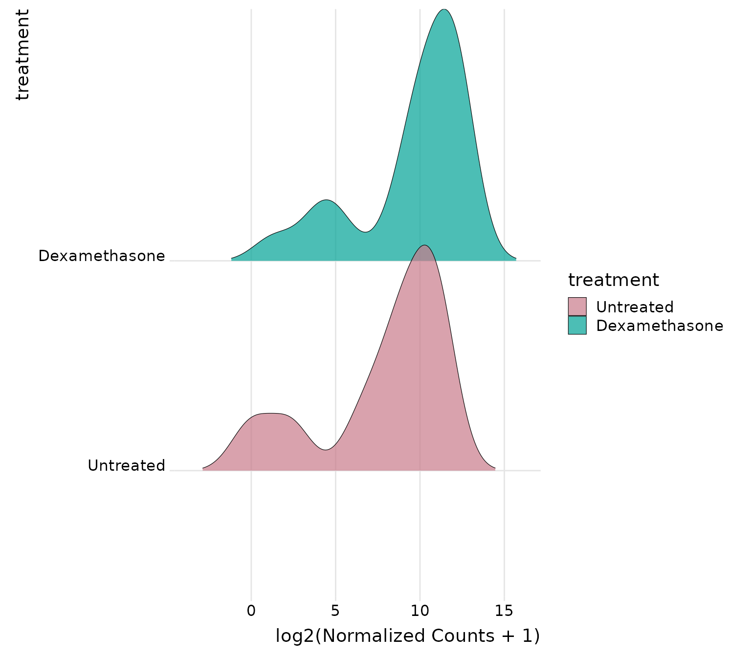
Joyplot by treatment group
# Ridges by treatment group - shows distribution for each group
get_expression_joyplot(
  vista,
  genes = top_up[1:5],
  log_transform = TRUE,
  y_by = "group",      # Each treatment group gets a ridge
  color_by = "group"   # Color by treatment group
)
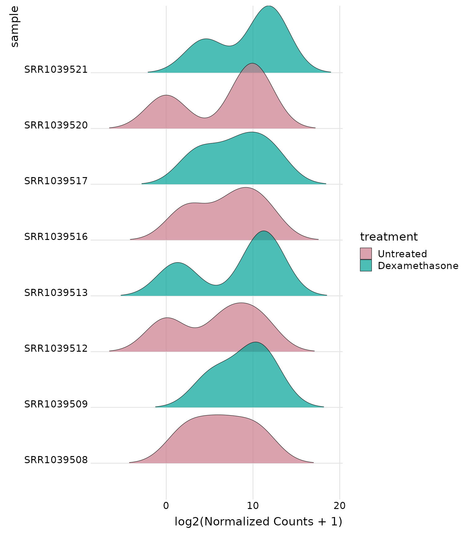
Joyplot by sample
# Ridges by individual sample - shows distribution for each sample
get_expression_joyplot(
  vista,
  genes = top_up[1:3],
  log_transform = TRUE,
  y_by = "sample",     # Each sample gets a ridge
  color_by = "group"   # Color by treatment group
)
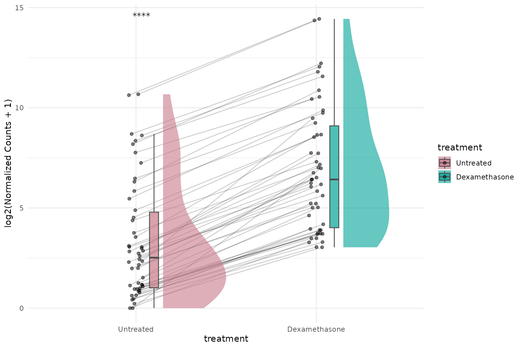
Raincloud plot (expression)
get_expression_raincloud(
  vista,
  genes = top_up,
  value_transform = "log2",
  summarise = TRUE,
  facet_by = "none",
  id.long.var = "gene",
  stats_group = TRUE
)
Functional Enrichment Analysis
MSigDB Enrichment
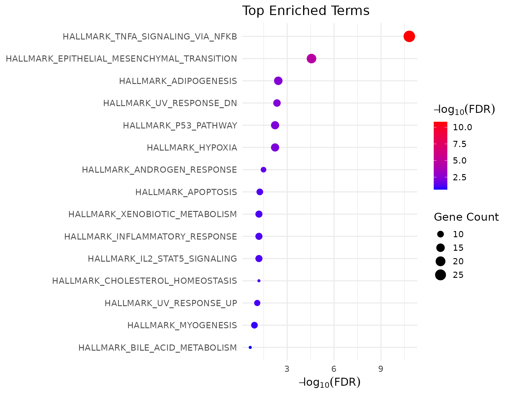
Hallmark gene sets - Upregulated
msig_up <- get_msigdb_enrichment(
vista,
sample_comparison = comp_names[1],
regulation = "Up",
msigdb_category = "H", # Hallmark gene sets
species = "Homo sapiens",
from_type = "ENSEMBL"
)
# View top enriched pathways
if (!is.null(msig_up$enrich) && nrow(msig_up$enrich@result) > 0) {
head(msig_up$enrich@result[, c("Description", "pvalue", "p.adjust", "Count")])
}
#> Description
#> HALLMARK_TNFA_SIGNALING_VIA_NFKB HALLMARK_TNFA_SIGNALING_VIA_NFKB
#> HALLMARK_EPITHELIAL_MESENCHYMAL_TRANSITION HALLMARK_EPITHELIAL_MESENCHYMAL_TRANSITION
#> HALLMARK_ADIPOGENESIS HALLMARK_ADIPOGENESIS
#> HALLMARK_UV_RESPONSE_DN HALLMARK_UV_RESPONSE_DN
#> HALLMARK_HYPOXIA HALLMARK_HYPOXIA
#> HALLMARK_P53_PATHWAY HALLMARK_P53_PATHWAY
#> pvalue p.adjust Count
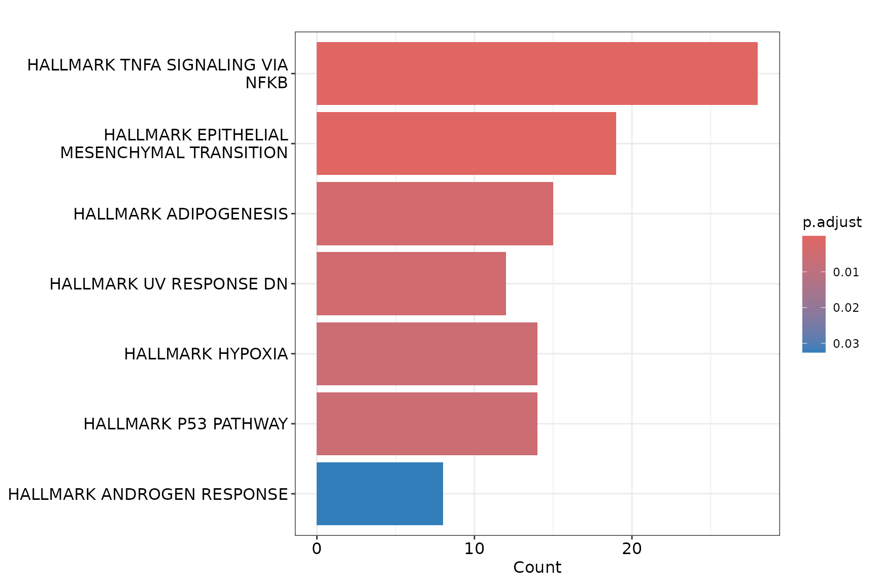
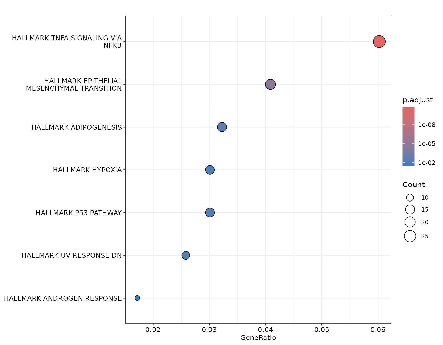
#> HALLMARK_TNFA_SIGNALING_VIA_NFKB 3.153757e-13 1.545341e-11 28
#> HALLMARK_EPITHELIAL_MESENCHYMAL_TRANSITION 1.136118e-06 2.783488e-05 19
#> HALLMARK_ADIPOGENESIS 2.272727e-04 3.712120e-03 15
#> HALLMARK_UV_RESPONSE_DN 3.664291e-04 4.488757e-03 12
#> HALLMARK_HYPOXIA 7.260526e-04 5.929430e-03 14
#> HALLMARK_P53_PATHWAY 7.260526e-04 5.929430e-03 14Hallmark gene sets - Downregulated
msig_down <- get_msigdb_enrichment(
  vista,
  sample_comparison = comp_names[1],
  regulation = "Down",
  msigdb_category = "H",
  species = "Homo sapiens",
  from_type = "ENSEMBL"
)

if (!is.null(msig_down$enrich) && nrow(msig_down$enrich@result) > 0) {
  head(msig_down$enrich@result[, c("Description", "pvalue", "p.adjust", "Count")])
}
#>                                                                           Description
#> HALLMARK_P53_PATHWAY                                             HALLMARK_P53_PATHWAY
#> HALLMARK_TNFA_SIGNALING_VIA_NFKB                     HALLMARK_TNFA_SIGNALING_VIA_NFKB
#> HALLMARK_EPITHELIAL_MESENCHYMAL_TRANSITION HALLMARK_EPITHELIAL_MESENCHYMAL_TRANSITION
#> HALLMARK_MTORC1_SIGNALING                                   HALLMARK_MTORC1_SIGNALING
#> HALLMARK_MYOGENESIS                                               HALLMARK_MYOGENESIS
#> HALLMARK_APOPTOSIS                                                 HALLMARK_APOPTOSIS
#>                                                  pvalue     p.adjust Count
#> HALLMARK_P53_PATHWAY                       1.669778e-06 7.180044e-05    17
#> HALLMARK_TNFA_SIGNALING_VIA_NFKB           4.166736e-04 8.958483e-03    13
#> HALLMARK_EPITHELIAL_MESENCHYMAL_TRANSITION 1.377933e-03 1.975037e-02    12
#> HALLMARK_MTORC1_SIGNALING                  4.197724e-03 3.610043e-02    11
#> HALLMARK_MYOGENESIS                        4.197724e-03 3.610043e-02    11
#> HALLMARK_APOPTOSIS                         8.312106e-03 5.673959e-02     9
Enrichment Visualizations
VISTA dotplot (default)
# VISTA's wrapper function
if (!is.null(msig_up$enrich) && nrow(msig_up$enrich@result) > 0) {
  get_enrichment_plot(msig_up$enrich, top_n = 10)
}
Barplot (clusterProfiler native)
# Use generic barplot with enrichResult method
if (!is.null(msig_up$enrich) && nrow(msig_up$enrich@result) > 0) {
  barplot(msig_up$enrich, showCategory = 10)
}
Dotplot with customization
# Customized dotplot with more categories
if (!is.null(msig_up$enrich) && nrow(msig_up$enrich@result) > 0) {
  enrichplot::dotplot(msig_up$enrich, showCategory = 20, font.size = 12)
}
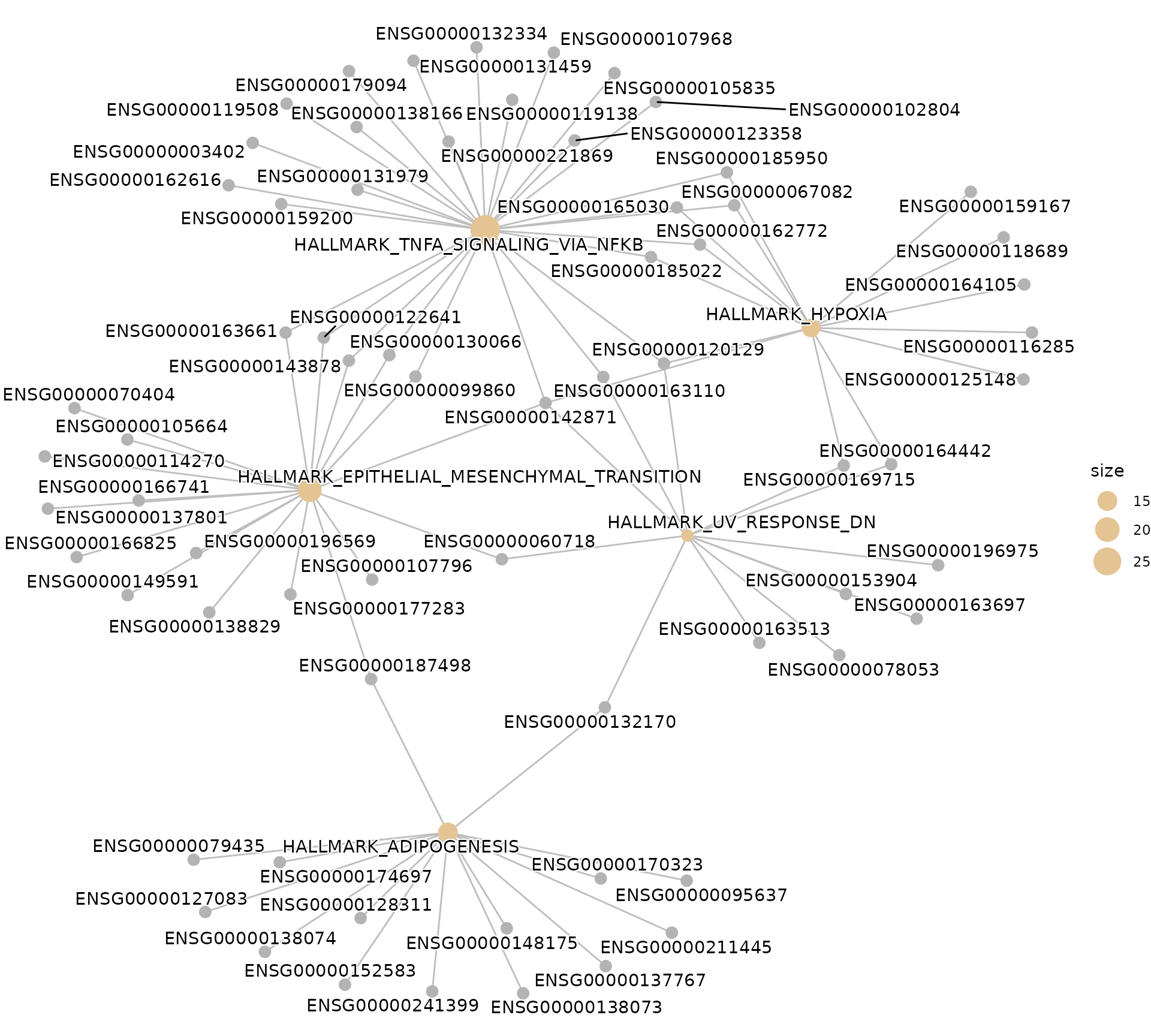
Network plot (clusterProfiler native)
# Gene-concept network showing gene-pathway relationships
if (!is.null(msig_up$enrich) && nrow(msig_up$enrich@result) > 0) {
  enrichplot::cnetplot(msig_up$enrich, showCategory = 5)
}
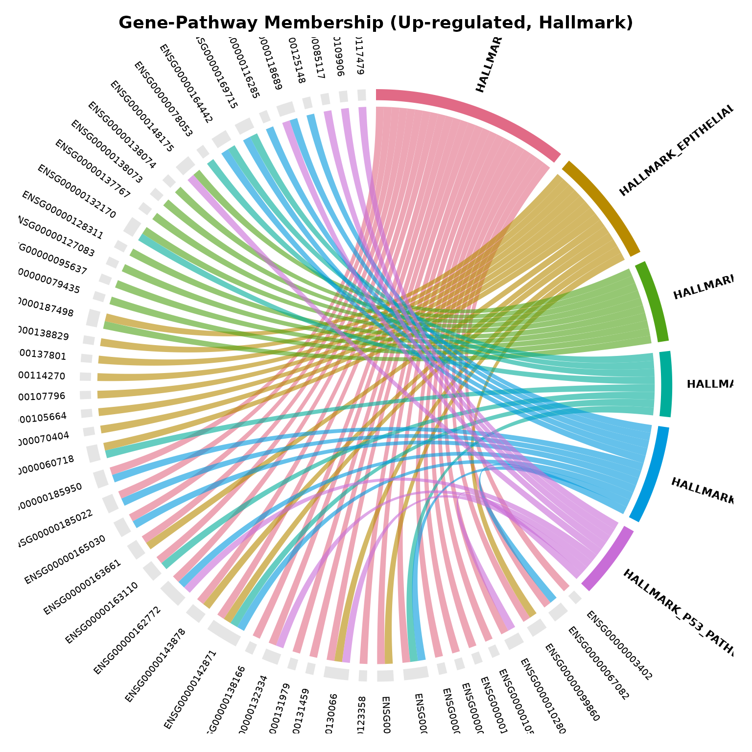
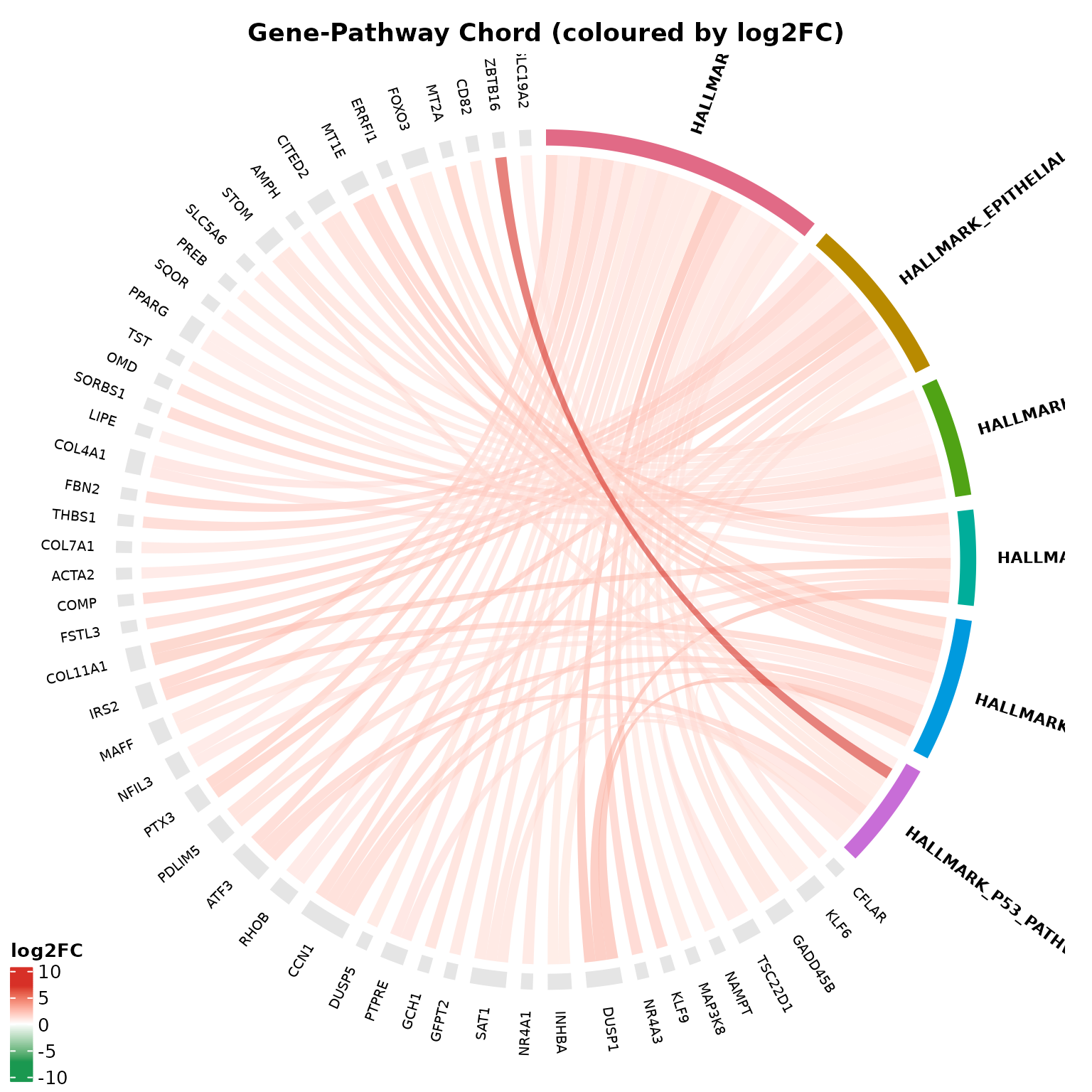
Chord diagram (gene–pathway relationships)
The chord diagram reveals which hub genes drive multiple enriched pathways and how much redundancy exists across terms. Chords can be coloured by fold-change when a VISTA object is supplied.
# Pathway-coloured chord diagram (no VISTA object needed)
if (!is.null(msig_up$enrich) && nrow(msig_up$enrich@result) > 0) {
  get_enrichment_chord(
    msig_up,
    top_n    = 6,
    color_by = "pathway",
    title    = "Gene-Pathway Membership (Up-regulated, Hallmark)"
  )
}
# Fold-change coloured chords
if (!is.null(msig_up$enrich) && nrow(msig_up$enrich@result) > 0) {
  get_enrichment_chord(
    msig_up,
    vista  = vista,
    sample_comparison = names(comparisons(vista))[1],
    top_n      = 6,
    color_by   = "foldchange",
    display_id = "SYMBOL",
    title      = "Gene-Pathway Chord (coloured by log2FC)"
  )
}
# Show only hub genes shared across 2+ pathways
if (!is.null(msig_up$enrich) && nrow(msig_up$enrich@result) > 0) {
  chord_result <- get_enrichment_chord(
    msig_up,
    vista    = vista,
    sample_comparison   = names(comparisons(vista))[1],
    top_n        = 8,
    min_pathways = 2,
    color_by     = "regulation",
    display_id   = "SYMBOL",
    title        = "Hub Genes Bridging Multiple Pathways"
  )

  # Inspect hub genes returned invisibly
  if (length(chord_result$hub_genes)) {
    cat("Hub genes:", paste(head(chord_result$hub_genes, 10), collapse = ", "), "\n")
  }
}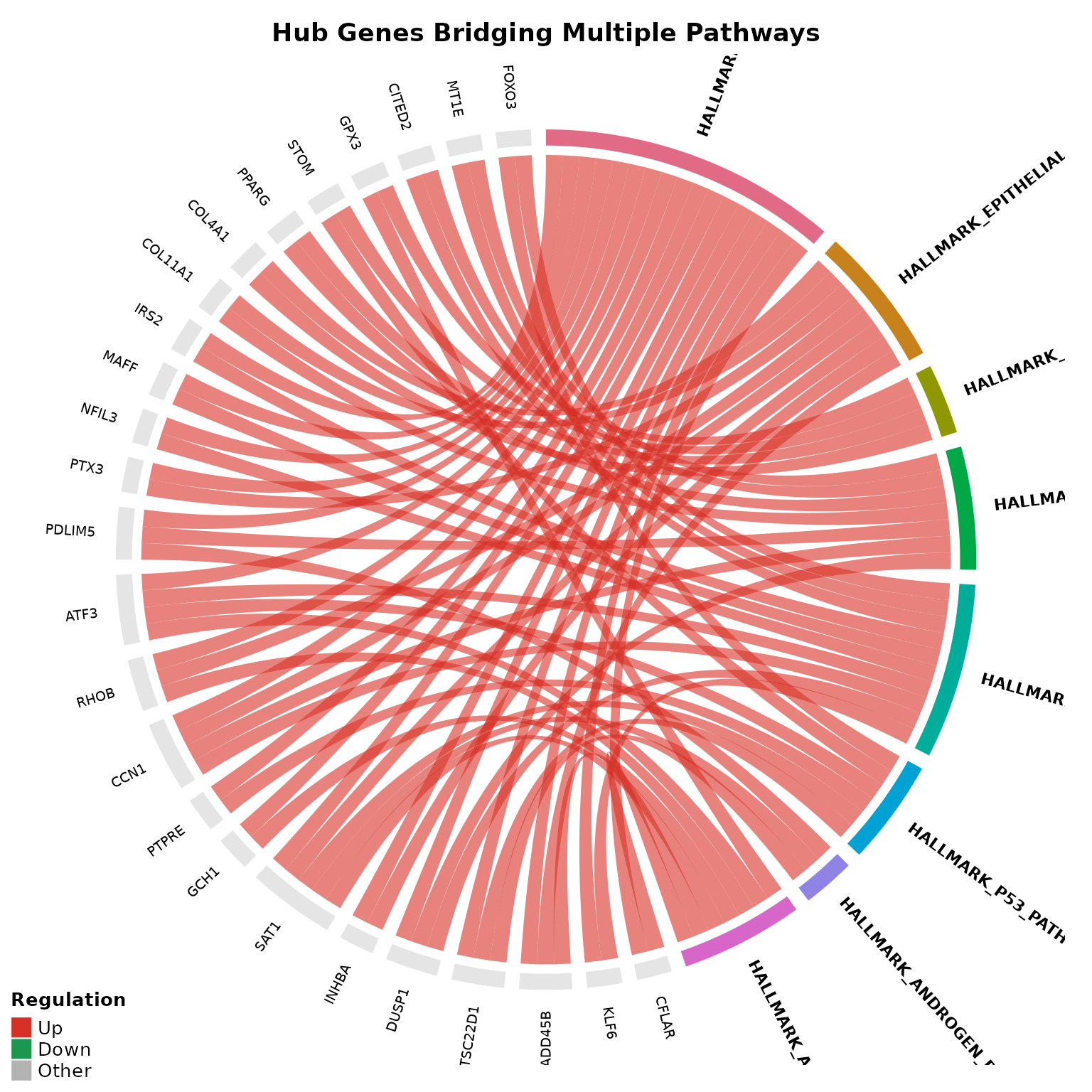
#> Hub genes: ENSG00000003402, ENSG00000060718, ENSG00000067082, ENSG00000099860, ENSG00000102804, ENSG00000118689, ENSG00000120129, ENSG00000122641, ENSG00000130066, ENSG00000131979Pathway-Specific Expression Heatmaps
Use enrichment output to extract pathway genes and visualize their expression directly.
Extract genes from top pathways
if (!is.null(msig_up$enrich) && nrow(msig_up$enrich@result) > 0) {
pathway_gene_list <- get_pathway_genes(
msig_up$enrich,
top_n = 3,
return_type = "list"
)
# Preview first few genes per pathway
lapply(pathway_gene_list, head, n = 5)
}
#> $HALLMARK_TNFA_SIGNALING_VIA_NFKB
#> [1] "ENSG00000003402" "ENSG00000067082" "ENSG00000099860" "ENSG00000102804"
#> [5] "ENSG00000105835"
#>
#> $HALLMARK_EPITHELIAL_MESENCHYMAL_TRANSITION
#> [1] "ENSG00000060718" "ENSG00000070404" "ENSG00000099860" "ENSG00000105664"
#> [5] "ENSG00000107796"
#>
#> $HALLMARK_ADIPOGENESIS
#> [1] "ENSG00000079435" "ENSG00000095637" "ENSG00000127083" "ENSG00000128311"
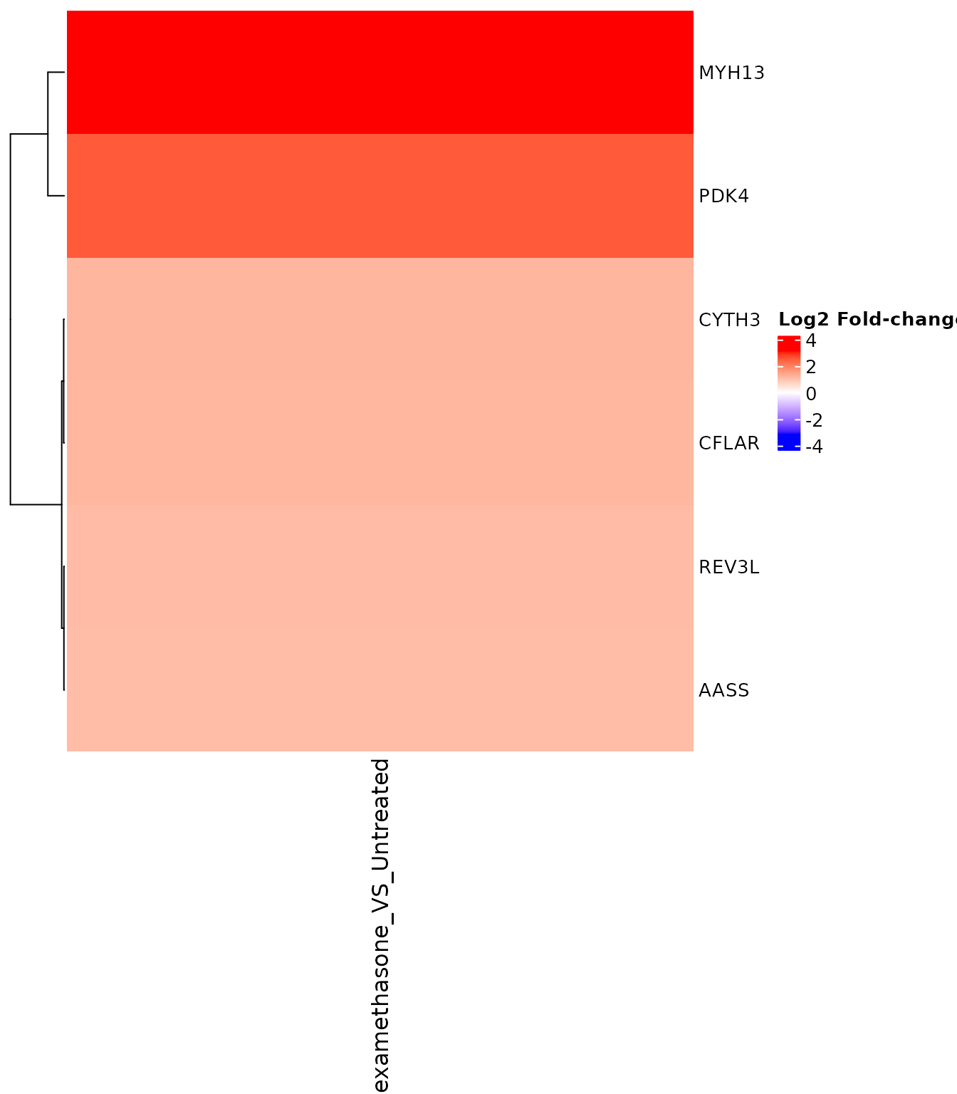
#> [5] "ENSG00000132170"Heatmap of genes from top enriched pathways
if (!is.null(msig_up$enrich) && nrow(msig_up$enrich@result) > 0) {
  get_pathway_heatmap(
    x = vista,
    enrichment = msig_up$enrich,
    sample_group = c("Untreated", "Dexamethasone"),
    top_n = 2,
    gene_mode = "union",
    max_genes = 60,
    value_transform = "zscore",
    display_id = "SYMBOL",
    annotate_columns = TRUE,
    summarise_replicates = FALSE,
    show_row_names = FALSE
  )
}
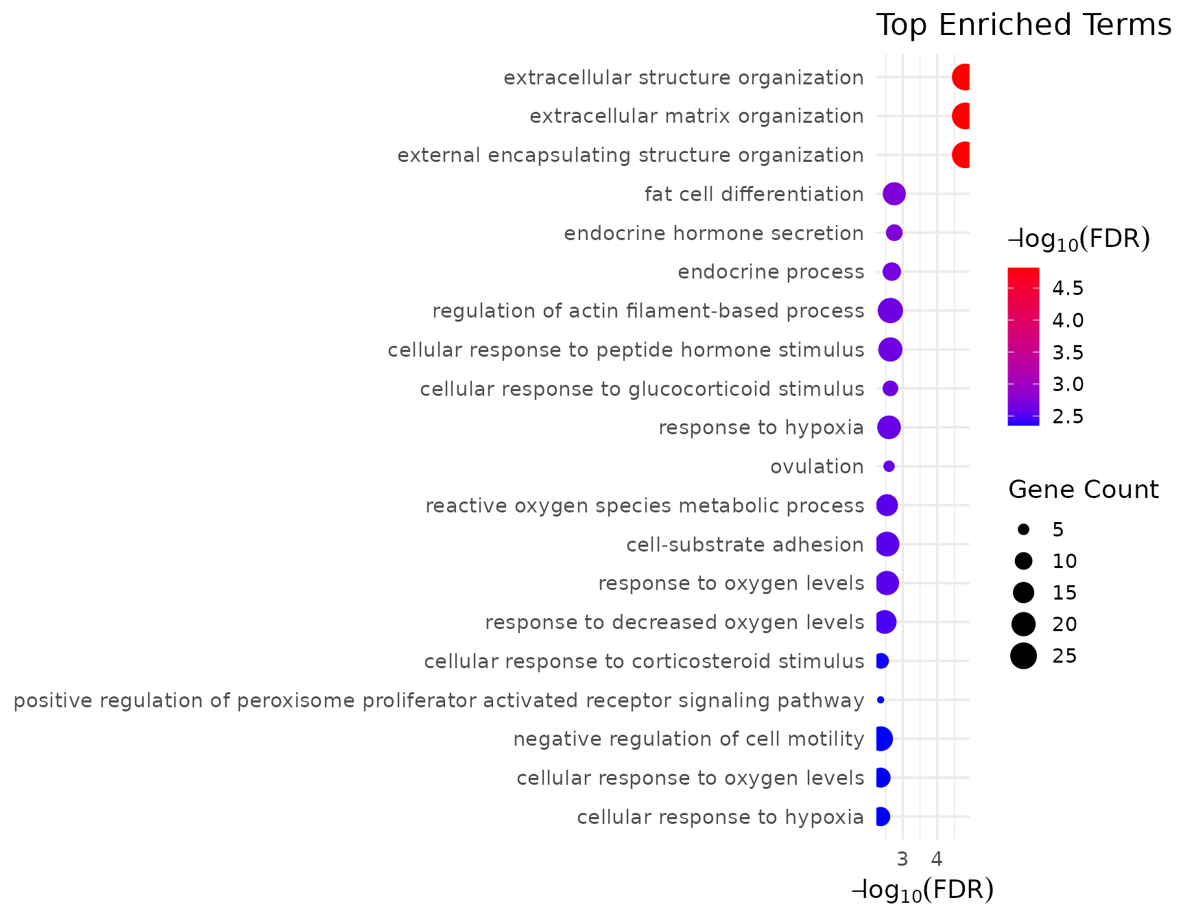
GO Enrichment
Biological Process
go_bp <- get_go_enrichment(
  vista,
  sample_comparison = comp_names[1],
  regulation = "Up",
  ont = "BP",  # Biological Process
  species = "Homo sapiens",
  from_type = "ENSEMBL"
)

if (!is.null(go_bp$enrich) && nrow(go_bp$enrich@result) > 0) {
  head(go_bp$enrich@result[, c("Description", "pvalue", "p.adjust", "Count")], n = 10)
}
#>                                              Description       pvalue
#> GO:0030198             extracellular matrix organization 1.060237e-08
#> GO:0043062          extracellular structure organization 1.116425e-08
#> GO:0045229 external encapsulating structure organization 1.237228e-08
#> GO:0060986                   endocrine hormone secretion 2.055554e-06
#> GO:0045444                      fat cell differentiation 2.395697e-06
#> GO:0050886                             endocrine process 3.389345e-06
#> GO:0071375 cellular response to peptide hormone stimulus 4.450874e-06
#> GO:0071385  cellular response to glucocorticoid stimulus 5.579975e-06
#> GO:0032970    regulation of actin filament-based process 5.601446e-06
#> GO:0030728                                     ovulation 6.962331e-06
#>                p.adjust Count
#> GO:0030198 1.531276e-05    25
#> GO:0043062 1.531276e-05    25
#> GO:0045229 1.531276e-05    25
#> GO:0060986 1.779044e-03     9
#> GO:0045444 1.779044e-03    18
#> GO:0050886 2.097440e-03    11
#> GO:0071375 2.310908e-03    20
#> GO:0071385 2.310908e-03     8
#> GO:0032970 2.310908e-03    22
#> GO:0030728 2.526439e-03     5
GO Visualization
if (!is.null(go_bp$enrich) && nrow(go_bp$enrich@result) > 0) {
  get_enrichment_plot(go_bp$enrich, top_n = 20)
}
Gene Set Enrichment Analysis (GSEA)
GSEA uses ranked gene lists to identify pathways enriched at the top or bottom of the ranking. VISTA automatically prepares the ranked list from your differential expression results.
GSEA with MSigDB Hallmark gene sets
# Run GSEA using VISTA's native function
gsea_results <- get_gsea(
vista,
sample_comparison = comp_names[1],
set_type = "msigdb",
from_type = "ENSEMBL",
species = "Homo sapiens",
msigdb_category = "H", # Hallmark gene sets
pvalueCutoff = 0.05,
pAdjustMethod = "BH"
)
# Show results
if (!is.null(gsea_results$enrich) && nrow(gsea_results$enrich@result) > 0) {
head(gsea_results$enrich@result[, c("Description", "NES", "pvalue", "p.adjust")], n = 10)
}
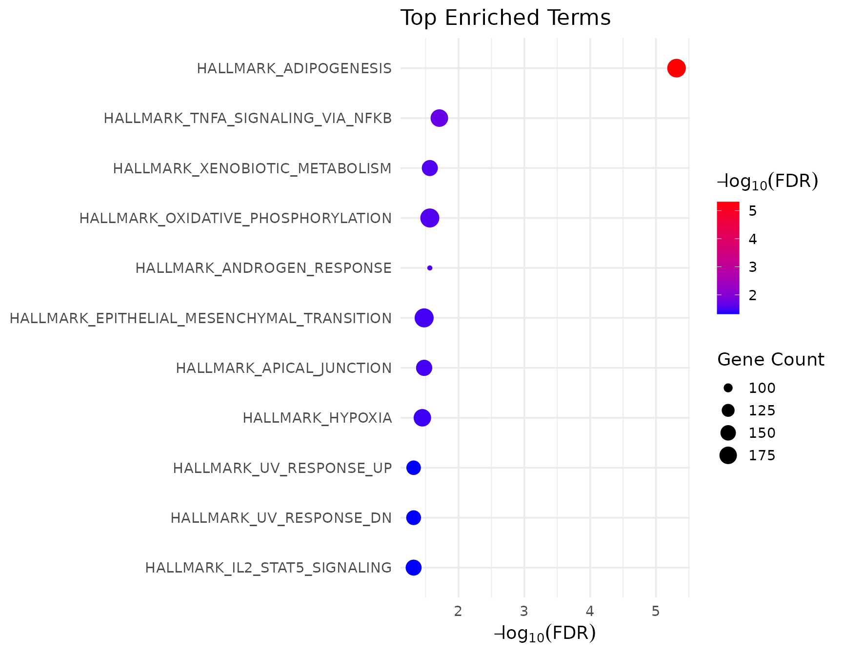
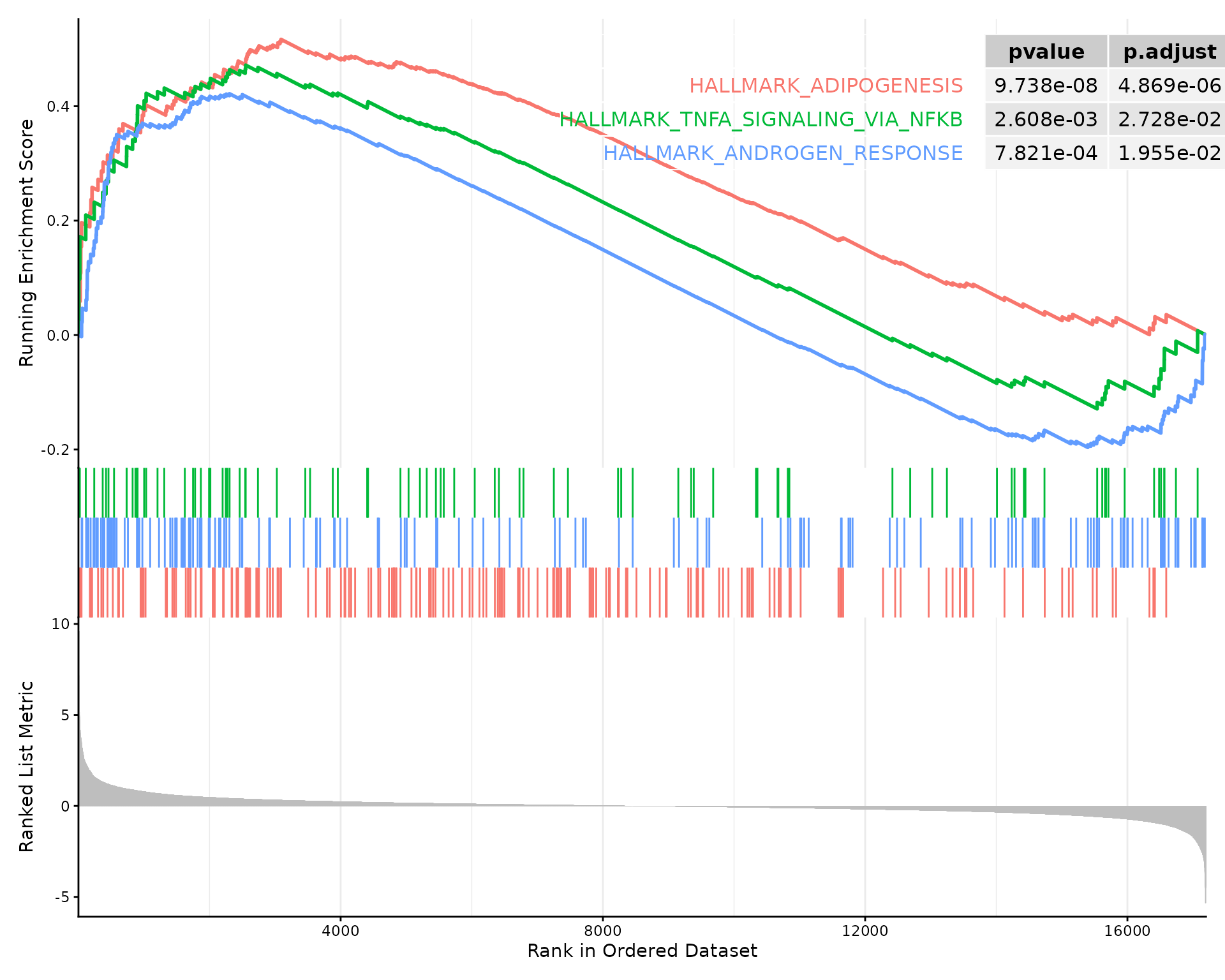
#> Description NES
#> HALLMARK_ADIPOGENESIS HALLMARK_ADIPOGENESIS 1.998365
#> HALLMARK_TNFA_SIGNALING_VIA_NFKB HALLMARK_TNFA_SIGNALING_VIA_NFKB 1.614221
#> HALLMARK_ANDROGEN_RESPONSE HALLMARK_ANDROGEN_RESPONSE 1.641697
#> HALLMARK_XENOBIOTIC_METABOLISM HALLMARK_XENOBIOTIC_METABOLISM 1.524633
#> HALLMARK_OXIDATIVE_PHOSPHORYLATION HALLMARK_OXIDATIVE_PHOSPHORYLATION 1.511488
#> pvalue p.adjust
#> HALLMARK_ADIPOGENESIS 3.106429e-08 1.553214e-06
#> HALLMARK_TNFA_SIGNALING_VIA_NFKB 6.454953e-04 1.613738e-02
#> HALLMARK_ANDROGEN_RESPONSE 2.151621e-03 3.064754e-02
#> HALLMARK_XENOBIOTIC_METABOLISM 3.064754e-03 3.064754e-02
#> HALLMARK_OXIDATIVE_PHOSPHORYLATION 2.575969e-03 3.064754e-02GSEA with GO Biological Process
# Run GSEA with GO terms
gsea_go <- get_gsea(
vista,
sample_comparison = comp_names[1],
set_type = "go",
from_type = "ENSEMBL",
orgdb = org.Hs.eg.db,
ont = "BP", # Biological Process
pvalueCutoff = 0.05
)
# Show results
if (!is.null(gsea_go$enrich) && nrow(gsea_go$enrich@result) > 0) {
head(gsea_go$enrich@result[, c("Description", "NES", "pvalue", "p.adjust")], n = 10)
}
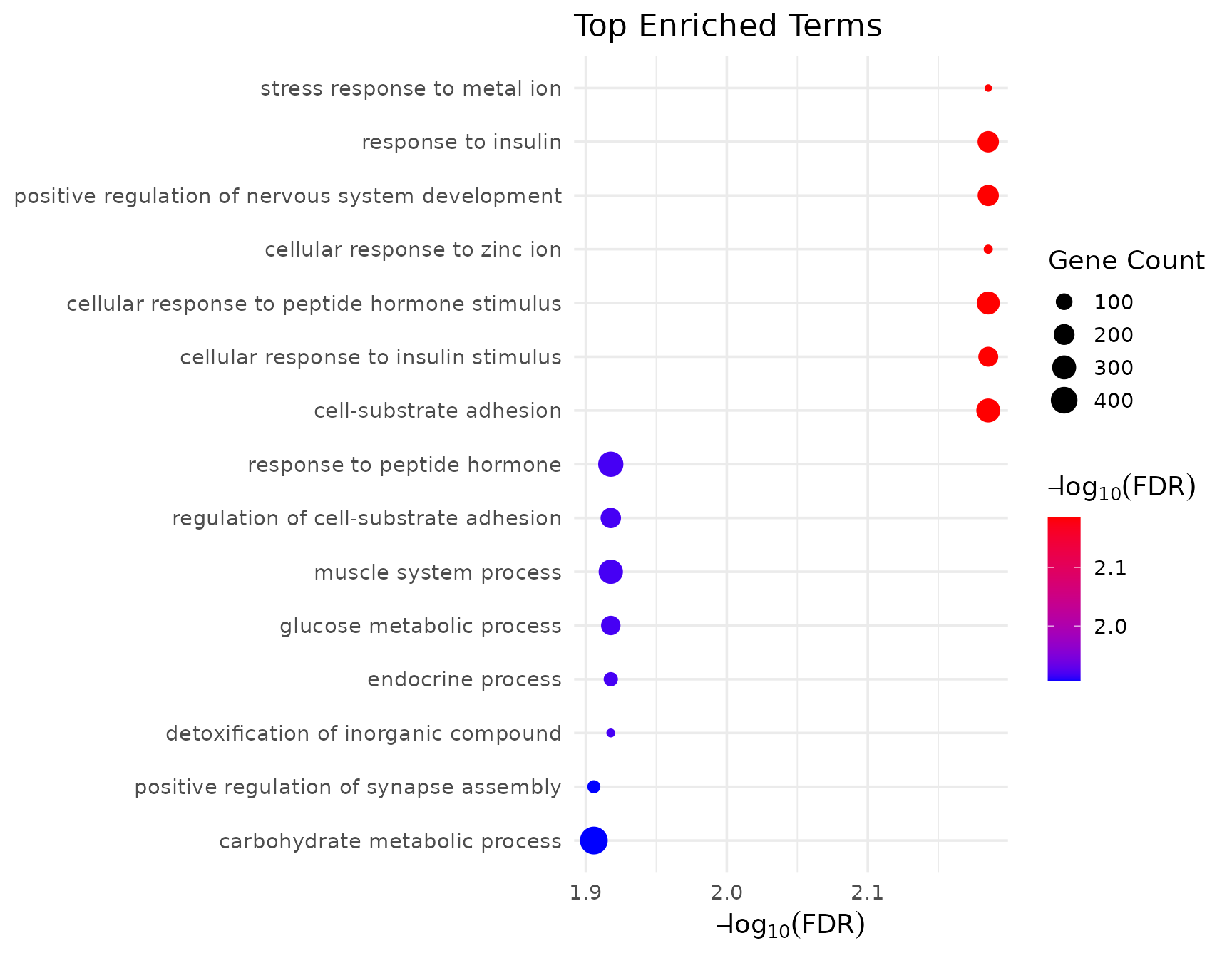
#> Description NES
#> GO:0071375 cellular response to peptide hormone stimulus 1.808024
#> GO:0051962 positive regulation of nervous system development -1.804617
#> GO:0071294 cellular response to zinc ion 2.041243
#> GO:0032869 cellular response to insulin stimulus 1.860517
#> GO:0006006 glucose metabolic process 1.821010
#> GO:0032868 response to insulin 1.807115
#> GO:0031589 cell-substrate adhesion 1.711791
#> GO:0003012 muscle system process 1.683786
#> GO:0097501 stress response to metal ion 1.994020
#> GO:0010810 regulation of cell-substrate adhesion 1.797353
#> pvalue p.adjust
#> GO:0071375 1.065356e-06 0.004144288
#> GO:0051962 1.518332e-06 0.004144288
#> GO:0071294 6.069393e-06 0.005262651
#> GO:0032869 4.035762e-06 0.005262651
#> GO:0006006 7.439886e-06 0.005262651
#> GO:0032868 7.712257e-06 0.005262651
#> GO:0031589 7.193516e-06 0.005262651
#> GO:0003012 5.540660e-06 0.005262651
#> GO:0097501 1.429395e-05 0.008670075
#> GO:0010810 1.786971e-05 0.009755073GSEA enrichment overview
# Show all significant pathways using VISTA's visualization
if (!is.null(gsea_results$enrich) && nrow(gsea_results$enrich@result) > 0) {
  get_enrichment_plot(gsea_results$enrich, top_n = 15)
}
GSEA plot for top pathway
# Show enrichment plot for the top pathway
if (!is.null(gsea_results$enrich) && nrow(gsea_results$enrich@result) > 0) {
  # Create GSEA enrichment plot with running enrichment score
  enrichplot::gseaplot2(
    gsea_results$enrich,
    geneSetID = 1,  # Top pathway
    title = gsea_results$enrich@result$Description[1],
    pvalue_table = TRUE
  )
}
GSEA plot for multiple pathways
# Show top 3 pathways together
if (!is.null(gsea_results$enrich) && nrow(gsea_results$enrich@result) > 0) {
  enrichplot::gseaplot2(
    gsea_results$enrich,
    geneSetID = 1:3,  # Top 3 pathways
    pvalue_table = TRUE,
    ES_geom = "line"
  )
}
GSEA with GO visualization
# Visualize GO GSEA results
if (!is.null(gsea_go$enrich) && nrow(gsea_go$enrich@result) > 0) {
  get_enrichment_plot(gsea_go$enrich, top_n = 15)
}
KEGG Pathway Enrichment
KEGG upregulated genes
kegg_up <- get_kegg_enrichment(
  vista,
  sample_comparison = comp_names[1],
  regulation = "Up",
  species = "Homo sapiens",
  from_type = "ENSEMBL"
)

if (!is.null(kegg_up$enrich) && nrow(kegg_up$enrich@result) > 0) {
  head(kegg_up$enrich@result[, c("Description", "pvalue", "p.adjust", "Count")], n = 10)
}
KEGG downregulated genes
kegg_down <- get_kegg_enrichment(
  vista,
  sample_comparison = comp_names[1],
  regulation = "Down",
  species = "Homo sapiens",
  from_type = "ENSEMBL"
)

if (!is.null(kegg_down$enrich) && nrow(kegg_down$enrich@result) > 0) {
  head(kegg_down$enrich@result[, c("Description", "pvalue", "p.adjust", "Count")])
}
KEGG Visualization
if (!is.null(kegg_up$enrich) && nrow(kegg_up$enrich@result) > 0) {
  get_enrichment_plot(kegg_up$enrich, top_n = 15)
}
Fold-Change Analysis
Fold-change Matrix
Useful for comparing multiple comparisons:
fc_matrix <- get_foldchange_matrix(vista)
head(fc_matrix, n = 10)
#> Dexamethasone_VS_Untreated
#> ENSG00000000003 -0.38027500
#> ENSG00000000419 0.20227695
#> ENSG00000000457 0.03272066
#> ENSG00000000460 -0.11851609
#> ENSG00000000971 0.43942357
#> ENSG00000001036 -0.24322719
#> ENSG00000001084 -0.03060707
#> ENSG00000001167 -0.49118392
#> ENSG00000001460 -0.13476909
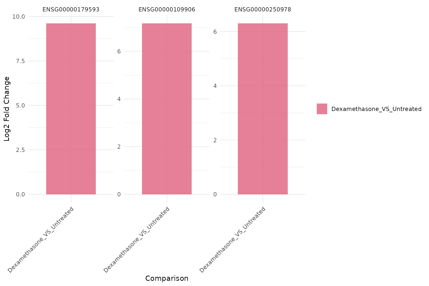
#> ENSG00000001461 -0.04363732Fold-change Barplot and Lollipop
Per-gene fold-change barplot
get_foldchange_barplot(
  vista,
  genes = top_up[1:3],
  sample_comparisons = comp_names,
  display_id = "SYMBOL",
  facet_by = "gene"
)
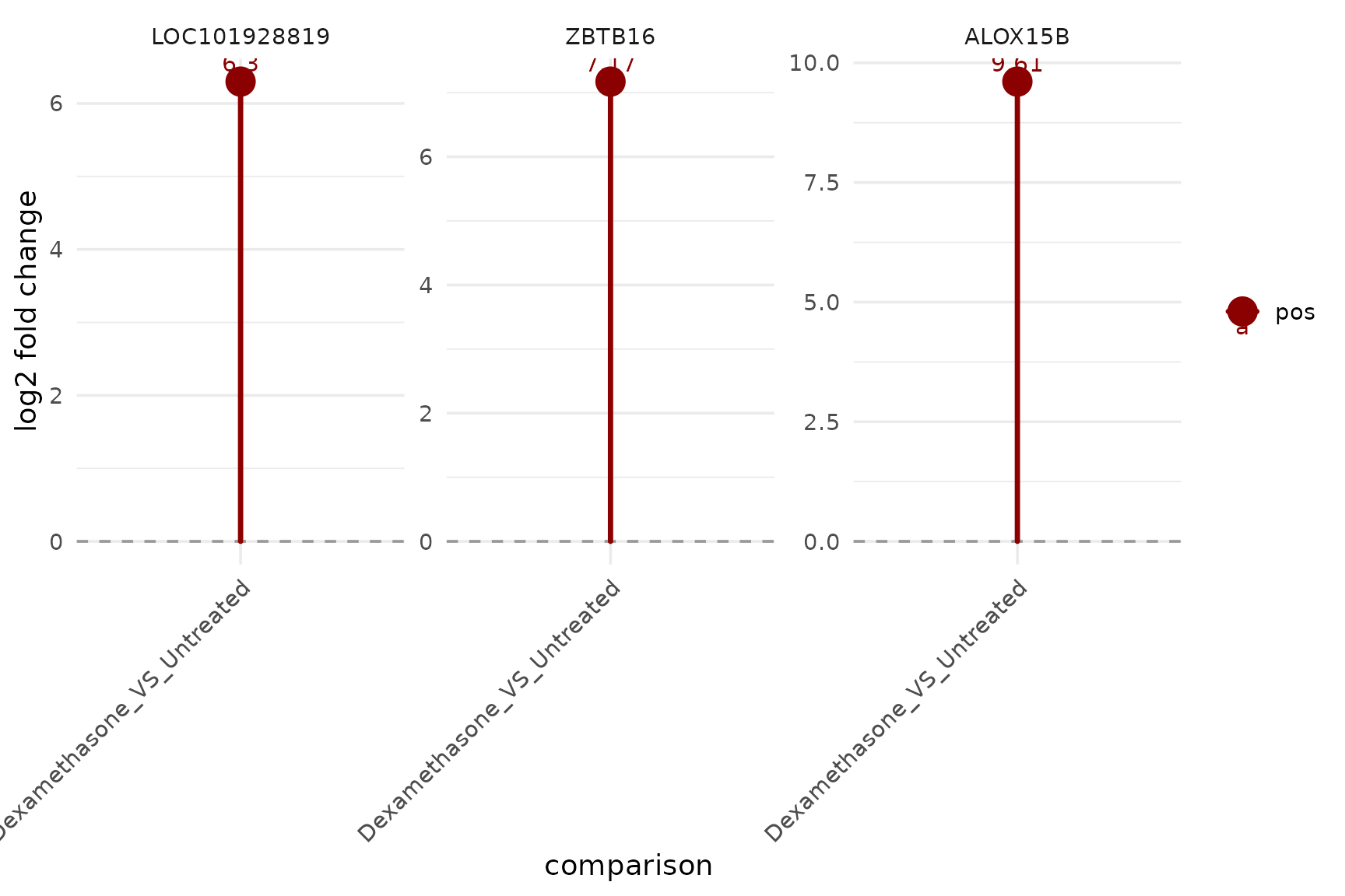
Per-gene fold-change lollipop
get_foldchange_lollipop(
  vista,
  sample_comparison = comp_names[1],
  genes = top_up[1:3],
  display_id = "SYMBOL",
  facet_by = "gene"
)
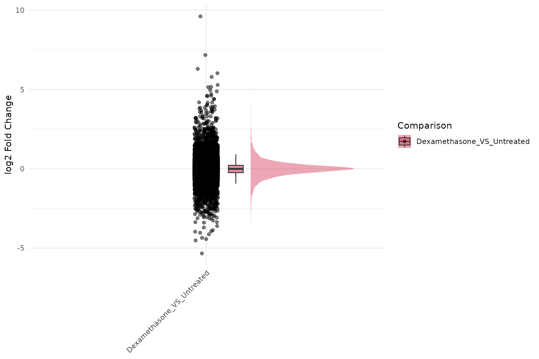
Fold-change Raincloud
get_foldchange_raincloud(
  vista,
  sample_comparisons = comp_names,
  facet_by = "none",
  id.long.var = "gene_id",
  stats_group = TRUE
)
Fold-change Heatmap
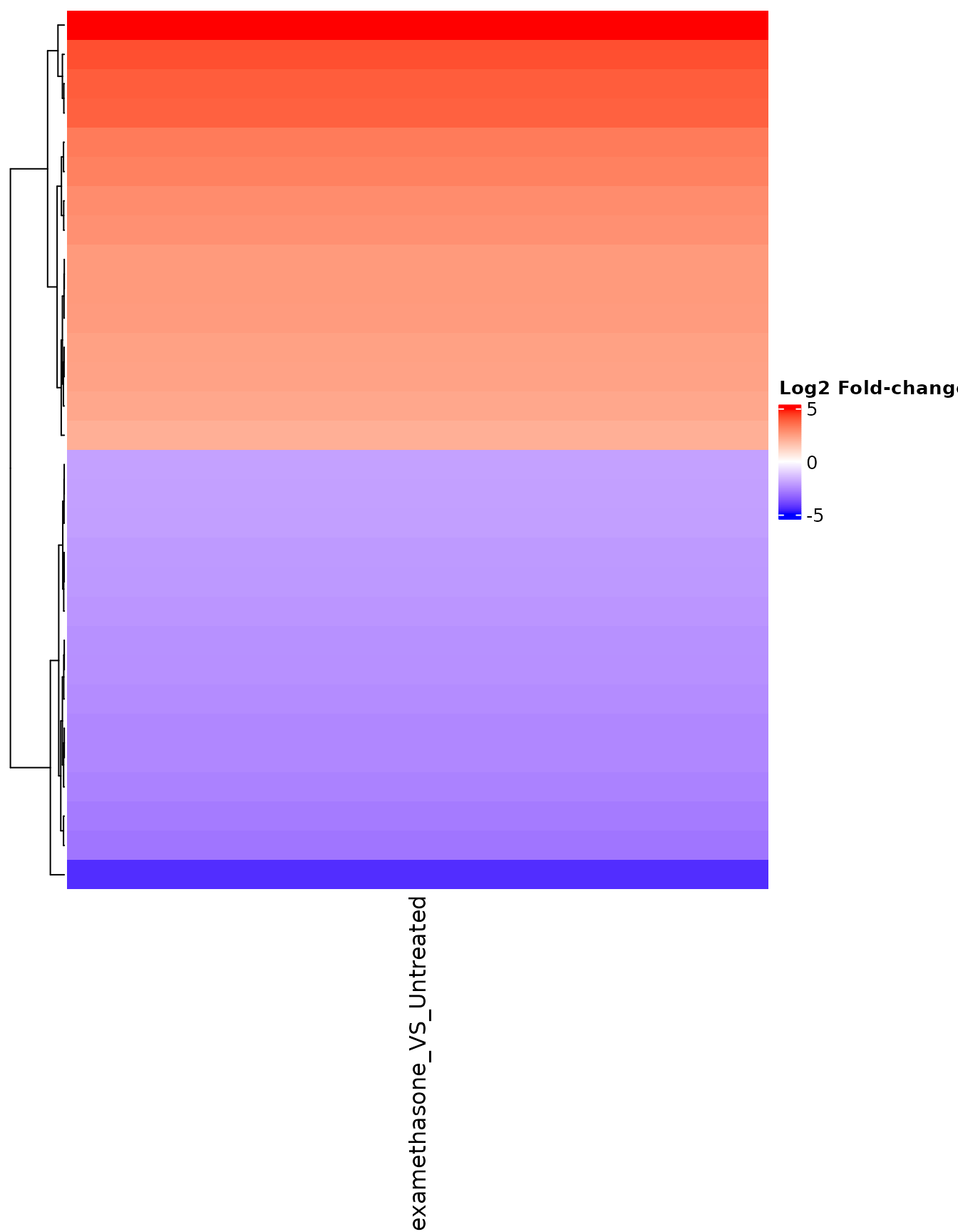
FC heatmap for selected genes
# Select genes with large fold-changes
fc_genes <- rownames(fc_matrix)[abs(fc_matrix[, 1]) > 2][1:30]

get_foldchange_heatmap(
  vista,
  sample_comparisons = comp_names,
  genes = fc_genes,
  display_id = "SYMBOL"
)
FC heatmap with gene names
get_foldchange_heatmap(
  vista,
  sample_comparisons = comp_names,
  genes = fc_genes[1:25],
  show_row_names = TRUE,
  display_id = "SYMBOL"
)
FC heatmap for specific gene set
# Use top upregulated genes
get_foldchange_heatmap(
  vista,
  sample_comparisons = comp_names,
  genes = top_up,
  show_row_names = TRUE,
  display_id = "SYMBOL"
)
Export Results
Export DE results to file
# Export complete DE table with annotations
de_annotated <- merge(
  comparisons(vista)[[1]],
  as.data.frame(rowData(vista)),
  by.x = "gene_id",
  by.y = "row.names"
)

# Write to CSV
write.csv(
  de_annotated,
  file = "airway_dexamethasone_vs_untreated_DE_results.csv",
  row.names = FALSE
)

# Export significant genes only
sig_genes <- de_annotated[de_annotated$regulation %in% c("Up", "Down"), ]
write.csv(
  sig_genes,
  file = "airway_significant_DEGs.csv",
  row.names = FALSE
)
Save VISTA object
# Save the complete VISTA object for later use
saveRDS(vista, file = "airway_vistaect.rds")

# Load it back
# vista <- readRDS("airway_vistaect.rds")
Summary
Workflow Completed
In this workflow, we:
- ✅ Loaded the airway RNA-seq dataset
- ✅ Created a VISTA object with DESeq2 analysis
- ✅ Added gene annotations from org.Hs.eg.db
- ✅ Performed quality control (PCA, MDS, UMAP, correlation)
- ✅ Visualized differential expression (volcano, MA plots)
- ✅ Analyzed expression patterns (heatmaps, barplots, boxplots, violin/raincloud plots, and more)
- ✅ Performed functional enrichment (MSigDB, GO, KEGG)
- ✅ Explored fold-change patterns
- ✅ Generated publication-ready visualizations
Key Features Demonstrated
-
Single-function workflow:
create_vista()handles DE analysis - Consistent interface: All plot functions follow the same pattern
- Flexible visualizations: Easy to customize colors, labels, thresholds
- Multiple plot types: 29+ plotting functions for every analysis need
- Integrated enrichment: No need to wrangle gene IDs manually
- Publication-ready: All plots are ggplot2/ComplexHeatmap objects
Plotting Functions Used
QC Plots
-
get_corr_heatmap()- Sample correlation -
get_pca_plot()- Principal component analysis -
get_mds_plot()- Multidimensional scaling -
get_umap_plot()- Nonlinear sample embedding
DE Visualization
-
get_deg_count_barplot()- DEG summary counts -
get_volcano_plot()- Volcano plots -
get_ma_plot()- MA plots
Expression Plots
-
get_expression_heatmap()- Expression heatmaps -
get_expression_barplot()- Expression barplots -
get_expression_boxplot()- Expression boxplots -
get_expression_violinplot()- Violin plots -
get_expression_density()- Density plots -
get_expression_scatter()- Sample-vs-sample scatter -
get_expression_lineplot()- Expression across samples -
get_expression_lollipop()- Lollipop plots -
get_expression_joyplot()- Ridgeline plots
Enrichment Plots
-
get_enrichment_plot()- Generic enrichment visualization -
get_msigdb_enrichment()- MSigDB enrichment -
get_go_enrichment()- GO enrichment -
get_kegg_enrichment()- KEGG pathway enrichment -
get_pathway_genes()- Extract genes driving enriched pathways -
get_pathway_heatmap()- Plot pathway-derived expression heatmaps -
get_enrichment_chord()- Chord diagram of gene-pathway relationships
Fold-Change
-
get_foldchange_matrix()- Extract FC matrix -
get_foldchange_heatmap()- Visualize FC patterns
Next Steps
- Try with your own data
- Explore edgeR backend:
method = "edger" - Explore limma-voom backend:
method = "limma" - Test multiple comparisons simultaneously
- Customize plots with ggplot2 themes
- Generate automated reports with
run_vista_report() - Integrate with downstream tools
Session Information
sessionInfo()
#> R version 4.5.3 (2026-03-11)
#> Platform: x86_64-pc-linux-gnu
#> Running under: Ubuntu 24.04.4 LTS
#>
#> Matrix products: default
#> BLAS:   /usr/lib/x86_64-linux-gnu/openblas-pthread/libblas.so.3
#> LAPACK: /usr/lib/x86_64-linux-gnu/openblas-pthread/libopenblasp-r0.3.26.so;  LAPACK version 3.12.0
#>
#> locale:
#>  [1] LC_CTYPE=C.UTF-8       LC_NUMERIC=C           LC_TIME=C.UTF-8
#>  [4] LC_COLLATE=C.UTF-8     LC_MONETARY=C.UTF-8    LC_MESSAGES=C.UTF-8
#>  [7] LC_PAPER=C.UTF-8       LC_NAME=C              LC_ADDRESS=C
#> [10] LC_TELEPHONE=C         LC_MEASUREMENT=C.UTF-8 LC_IDENTIFICATION=C
#>
#> time zone: UTC
#> tzcode source: system (glibc)
#>
#> attached base packages:
#> [1] stats4    stats     graphics  grDevices utils     datasets  methods
#> [8] base
#>
#> other attached packages:
#>  [1] magrittr_2.0.5              org.Hs.eg.db_3.22.0
#>  [3] AnnotationDbi_1.72.0        airway_1.30.0
#>  [5] SummarizedExperiment_1.40.0 Biobase_2.70.0
#>  [7] GenomicRanges_1.62.1        Seqinfo_1.0.0
#>  [9] IRanges_2.44.0              S4Vectors_0.49.1-1
#> [11] BiocGenerics_0.56.0         generics_0.1.4
#> [13] MatrixGenerics_1.22.0       matrixStats_1.5.0
#> [15] ggplot2_4.0.2               VISTA_0.99.8
#> [17] BiocStyle_2.38.0
#>
#> loaded via a namespace (and not attached):
#>   [1] splines_4.5.3           ggplotify_0.1.3         tibble_3.3.1
#>   [4] R.oo_1.27.1             ggpp_0.6.0              polyclip_1.10-7
#>   [7] lifecycle_1.0.5         rstatix_0.7.3           edgeR_4.8.2
#>  [10] doParallel_1.0.17       lattice_0.22-9          MASS_7.3-65
#>  [13] backports_1.5.1         limma_3.66.0            sass_0.4.10
#>  [16] rmarkdown_2.31          jquerylib_0.1.4         yaml_2.3.12
#>  [19] otel_0.2.0              ggtangle_0.1.1          EnhancedVolcano_1.28.2
#>  [22] cowplot_1.2.0           DBI_1.3.0               RColorBrewer_1.1-3
#>  [25] abind_1.4-8             purrr_1.2.2             R.utils_2.13.0
#>  [28] msigdbr_26.1.0          yulab.utils_0.2.4       tweenr_2.0.3
#>  [31] rappdirs_0.3.4          gdtools_0.5.0           circlize_0.4.18
#>  [34] enrichplot_1.30.5       ggrepel_0.9.8           tidytree_0.4.7
#>  [37] RSpectra_0.16-2         pkgdown_2.2.0           codetools_0.2-20
#>  [40] DelayedArray_0.36.1     DOSE_4.4.0              ggforce_0.5.0
#>  [43] tidyselect_1.2.1        shape_1.4.6.1           aplot_0.2.9
#>  [46] farver_2.1.2            jsonlite_2.0.0          GetoptLong_1.1.1
#>  [49] Formula_1.2-5           ggridges_0.5.7          iterators_1.0.14
#>  [52] systemfonts_1.3.2       foreach_1.5.2           tools_4.5.3
#>  [55] ggnewscale_0.5.2        treeio_1.34.0           ragg_1.5.2
#>  [58] Rcpp_1.1.1              glue_1.8.0              gridExtra_2.3
#>  [61] SparseArray_1.10.10     xfun_0.57               DESeq2_1.50.2
#>  [64] qvalue_2.42.0           dplyr_1.2.1             withr_3.0.2
#>  [67] BiocManager_1.30.27     fastmap_1.2.0           GGally_2.4.0
#>  [70] ggpointdensity_0.2.1    digest_0.6.39           R6_2.6.1
#>  [73] gridGraphics_0.5-1      textshaping_1.0.5       colorspace_2.1-2
#>  [76] GO.db_3.22.0            RSQLite_2.4.6           ggrain_0.1.2
#>  [79] R.methodsS3_1.8.2       tidyr_1.3.2             fontLiberation_0.1.0
#>  [82] data.table_1.18.2.1     FNN_1.1.4.1             httr_1.4.8
#>  [85] htmlwidgets_1.6.4       S4Arrays_1.10.1         scatterpie_0.2.6
#>  [88] ggstats_0.13.0          uwot_0.2.4              pkgconfig_2.0.3
#>  [91] gtable_0.3.6            blob_1.3.0              ComplexHeatmap_2.26.1
#>  [94] S7_0.2.1                XVector_0.50.0          clusterProfiler_4.18.4
#>  [97] htmltools_0.5.9         carData_3.0-6           fontBitstreamVera_0.1.1
#> [100] bookdown_0.46           fgsea_1.36.2            clue_0.3-68
#> [103] scales_1.4.0            png_0.1-9               ggfun_0.2.0
#> [106] knitr_1.51              reshape2_1.4.5          rjson_0.2.23
#> [109] nlme_3.1-168            curl_7.0.0              cachem_1.1.0
#> [112] GlobalOptions_0.1.4     stringr_1.6.0           parallel_4.5.3
#> [115] desc_1.4.3              pillar_1.11.1           grid_4.5.3
#> [118] vctrs_0.7.3             ggpubr_0.6.3            car_3.1-5
#> [121] tidydr_0.0.6            cluster_2.1.8.2         evaluate_1.0.5
#> [124] cli_3.6.6               locfit_1.5-9.12         compiler_4.5.3
#> [127] rlang_1.2.0             crayon_1.5.3            ggsignif_0.6.4
#> [130] labeling_0.4.3          forcats_1.0.1           plyr_1.8.9
#> [133] fs_2.0.1                ggiraph_0.9.6           stringi_1.8.7
#> [136] viridisLite_0.4.3       BiocParallel_1.44.0     assertthat_0.2.1
#> [139] babelgene_22.9          Biostrings_2.78.0       lazyeval_0.2.3
#> [142] GOSemSim_2.36.0         fontquiver_0.2.1        Matrix_1.7-4
#> [145] patchwork_1.3.2         bit64_4.6.0-1           KEGGREST_1.50.0
#> [148] statmod_1.5.1           broom_1.0.12            igraph_2.2.3
#> [151] memoise_2.0.1           bslib_0.10.0            ggtree_4.0.5
#> [154] fastmatch_1.1-8         bit_4.6.0               ape_5.8-1
#> [157] gson_0.1.0              polynom_1.4-1
References
- Himes BE et al. (2014). RNA-Seq Transcriptome Profiling Identifies CRISPLD2 as a Glucocorticoid Responsive Gene that Modulates Cytokine Function in Airway Smooth Muscle Cells. PLoS One, 9(6), e99625.
- Love MI, Huber W, Anders S (2014). Moderated estimation of fold change and dispersion for RNA-seq data with DESeq2. Genome Biology, 15, 550.
- Robinson MD, McCarthy DJ, Smyth GK (2010). edgeR: a Bioconductor package for differential expression analysis of digital gene expression data. Bioinformatics, 26(1), 139-140.
- Subramanian A et al. (2005). Gene set enrichment analysis: a knowledge-based approach for interpreting genome-wide expression profiles. PNAS, 102(43), 15545-15550.
- Yu G et al. (2012). clusterProfiler: an R package for comparing biological themes among gene clusters. OMICS, 16(5), 284-287.